1, Batch normalization and residual network

1.1 batch normalization

Standardization of inputs (shallow models)

• The mean value and standard deviation of any feature after processing on all samples in the data set are 0 and 1.
• Standardized processing of input data makes the distribution of each feature similar

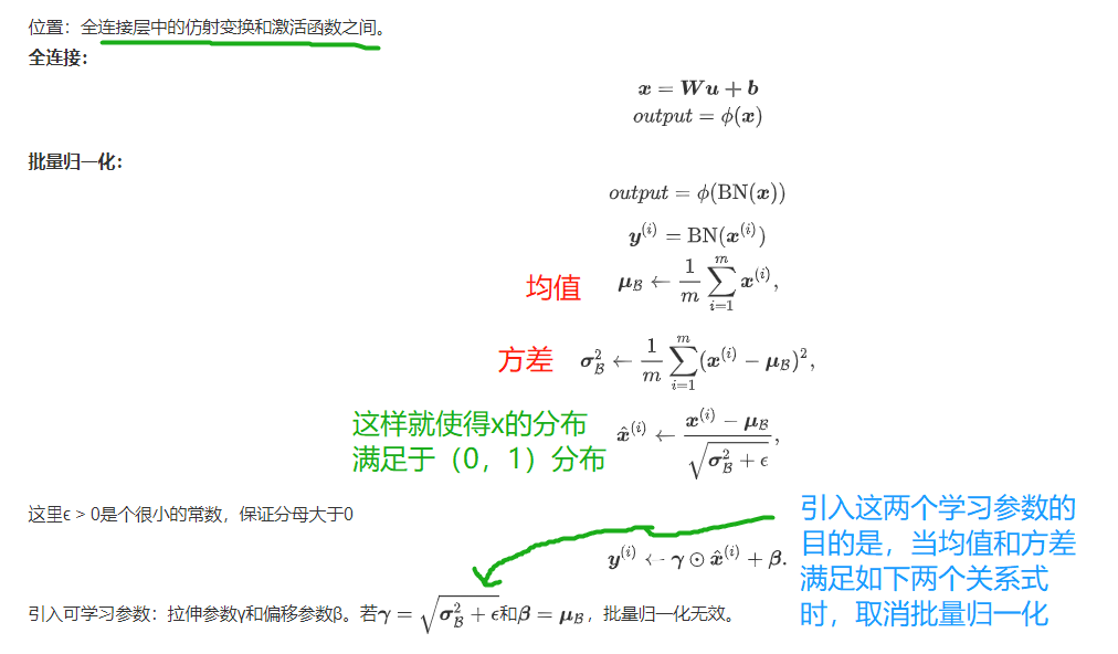
Batch normalization (depth model)
By using the mean and standard deviation of small batch, the intermediate output of the neural network is adjusted continuously, so that the value of the intermediate output of the whole neural network in each layer is more stable.

Batch reduction in forecast

Training: calculate the mean and variance of each batch in batch.
Prediction: the moving average is used to estimate the sample mean and variance of the whole training data set.

1.2 residual network (ResNet)

The problem of deep learning: after deep CNN network reaches a certain depth, increasing the number of layers again will not improve the classification performance, but will lead to slower network convergence and worse accuracy.

Residual Block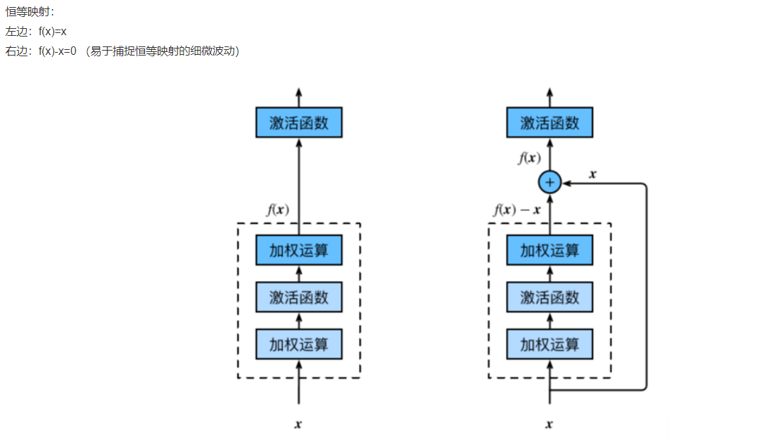

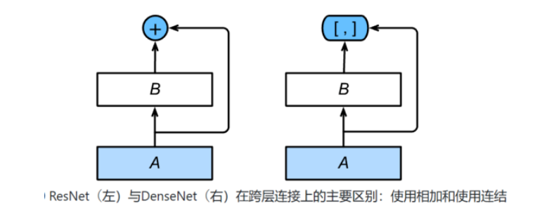
1.3 dense network

Main building blocks:
dense block: defines how input and output are connected, specifically the calculation method of output channel.
transition layer: use 1 × 1 convolution operation to control the number of channels, so that it is not large. At the same time, the average pool will be used to reduce the size.

#The code of dense block is as follows:
def conv_block(in_channels, out_channels):
    blk = nn.Sequential(nn.BatchNorm2d(in_channels), 
                        nn.ReLU(),
                        nn.Conv2d(in_channels, out_channels, kernel_size=3, padding=1))
    return blk

class DenseBlock(nn.Module):
    def __init__(self, num_convs, in_channels, out_channels):
        super(DenseBlock, self).__init__()
        net = []
        for i in range(num_convs):
            in_c = in_channels + i * out_channels
            net.append(conv_block(in_c, out_channels))
        self.net = nn.ModuleList(net)
        self.out_channels = in_channels + num_convs * out_channels ### Calculate the number of output channels

    def forward(self, X):
        for blk in self.net:
            Y = blk(X)
            X = torch.cat((X, Y), dim=1)  # Linking input and output in the channel dimension
        return X

#The code of the transition block is as follows:
def transition_block(in_channels, out_channels):
    blk = nn.Sequential(
            nn.BatchNorm2d(in_channels),  #normalization
            nn.ReLU(),  #Nonlinear activation function
            nn.Conv2d(in_channels, out_channels, kernel_size=1),  #1 × 1 convolution operation to reduce the number of channels
            nn.AvgPool2d(kernel_size=2, stride=2)) #Average pooling reduces output size
    return blk

2. Convex optimization

2.1 optimization and deep learning

Optimization and estimation
Although the optimization method can minimize the loss function value in deep learning, in essence, the goal of the optimization method is not the same as that of deep learning.

• Objective of optimization method: loss function value of training set
• Deep learning objective: test set loss function value (generalization)

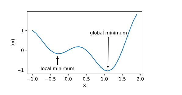
The challenge of optimization in deep learning

1. Local minimum
   
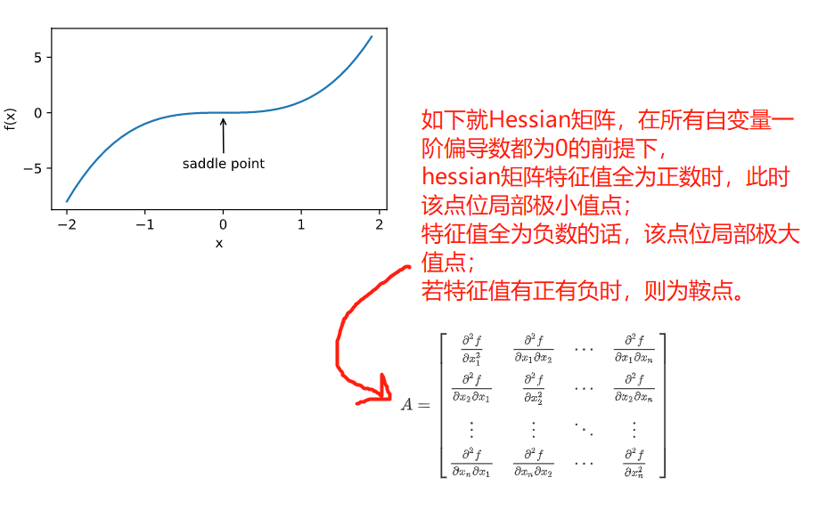
2. saddle point
   
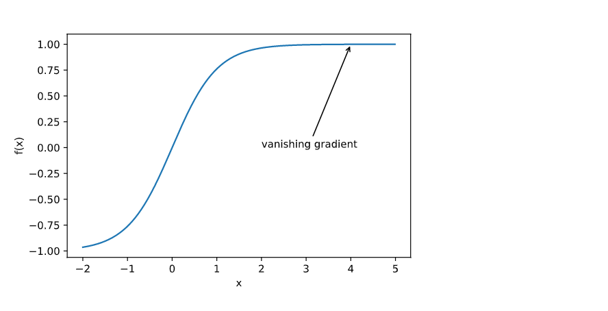
3. Gradient disappear
   

2.2 Convexity

Convex function set: if the connection of any two points in a set is in the set, it is called convex set.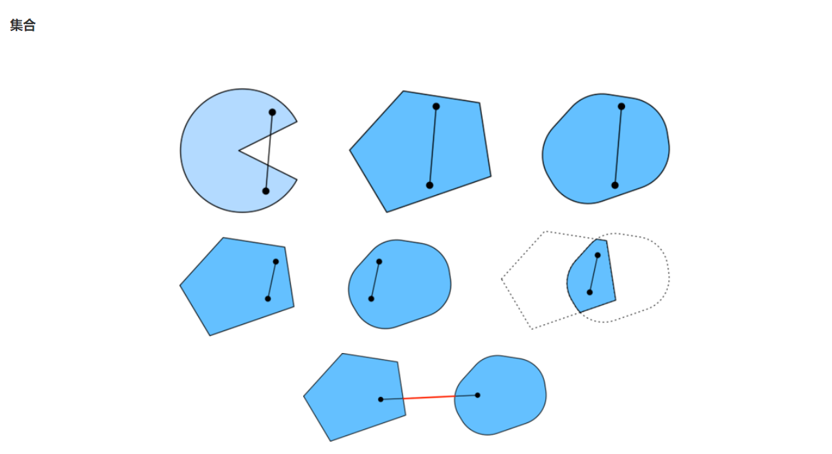

Nature

1. No local minimum
2. Relation with convex set
3. Two order condition

Proof: slightly

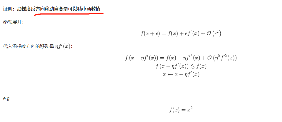
3. Gradient descent

3.1 one dimensional gradient descent

3.2 multidimensional gradient decline

3.3 simple implementation

# This function differs from the original book in that the first parameter optimizer function here is not the name of the optimizer
# For example: optimizer FN = torch. Optim. SGD, optimizer hyperparams = {"LR": 0.05}
def train_pytorch_ch7(optimizer_fn, optimizer_hyperparams, features, labels,
                    batch_size=10, num_epochs=2):
    # Initialize model
    net = nn.Sequential(
        nn.Linear(features.shape[-1], 1)
    )
    loss = nn.MSELoss()
    optimizer = optimizer_fn(net.parameters(), **optimizer_hyperparams)

    def eval_loss():
        return loss(net(features).view(-1), labels).item() / 2

    ls = [eval_loss()]
    data_iter = torch.utils.data.DataLoader(
        torch.utils.data.TensorDataset(features, labels), batch_size, shuffle=True)

    for _ in range(num_epochs):
        start = time.time()
        for batch_i, (X, y) in enumerate(data_iter):
            # Divide by 2 to be consistent with train ABCD 7, because in squared ABCD loss, except for 2
            l = loss(net(X).view(-1), y) / 2 
            
            optimizer.zero_grad()
            l.backward()
            optimizer.step()
            if (batch_i + 1) * batch_size % 100 == 0:
                ls.append(eval_loss())
    # Printing results and drawing
    print('loss: %f, %f sec per epoch' % (ls[-1], time.time() - start))
    d2l.set_figsize()
    d2l.plt.plot(np.linspace(0, num_epochs, len(ls)), ls)
    d2l.plt.xlabel('epoch')
    d2l.plt.ylabel('loss')
train_pytorch_ch7(optim.SGD, {"lr": 0.05}, features, labels, 10)

The content comes from the courseware of Boyu college, which is only used as its own learning record