sklearn provides one-class SVM and Elliptic Envelope for anomaly detection. The former is an unsupervised anomaly detection method based on libsvm, which can be used to evaluate high-dimensional distribution. The latter can only do anomaly detection based on Gauss distribution data set.

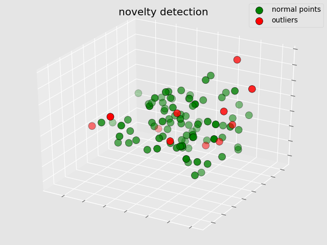
The example in this section simulates the training of anomaly detection model for a batch of raw data without any labels, and then discovers the anomaly data in the new data set through a new test set.

The red dots in the figure represent outliers and the green dots represent normal points. In python, the graphics can be dragged and dragged directly through the mouse to display the data distribution from different 3D perspectives, which is very useful when the points in some areas are relatively concentrated.

# Read the data file through Numpy's loadtxt.
# · Slice the matrix.
# · Using OneClassSVM method in sklearn.svm to realize anomaly detection and analysis, and using it
# fit method is applied to the training set and predict method is applied to the test set.
# · Numpy's hstack method is used to merge the matrices in columns to get a new matrix.
# · By judging the values of specific columns in the matrix, the data set can be directly selected or cut.
# · The shape of matrix is obtained by shape method.
# · The output is formatted by using print method and str.format.
# · The pre-defined library style of Matplotlib is used by plt.style.use method.
# · By using the Axes3D method of mpl_toolkits.mplot3d, 3D image conversion is done.
# · The scatter method of matplotlib.pyplot is used to draw scatter points, and the scatter method is used to display the scatter points.
# Set different display styles, including color, style, legend, etc. Aiming at and hiding coordinate axis labels, setting legends and labels, setting headings, etc.
import matplotlib
matplotlib.use('TkAgg')
# Import library
from sklearn.svm import OneClassSVM # Import OneClassSVM
import numpy as np # Import numpy Library
import matplotlib.pyplot as plt # Import Matplotlib
from mpl_toolkits.mplot3d import Axes3D # Import 3D Style Library
# Data preparation
raw_data = np.loadtxt('outlier.txt', delimiter=' ') # Read data
train_set = raw_data[:900, :] # training set
test_set = raw_data[:100, :] # Test set
# Abnormal Data Detection
model_onecalsssvm = OneClassSVM(nu=0.1, kernel="rbf", random_state=0) # Create anomaly detection algorithm model object
model_onecalsssvm.fit(train_set) # Training model
pre_test_outliers = model_onecalsssvm.predict(test_set) # anomaly detection
# Statistics of abnormal results
toal_test_data = np.hstack((test_set, pre_test_outliers.reshape(test_set.shape[0], 1))) # Merge test sets with test results
normal_test_data = toal_test_data[toal_test_data[:, -1] == 1] # Obtaining the set of abnormal detection results
outlier_test_data = toal_test_data[toal_test_data[:, -1] == -1] # Obtaining abnormal data of abnormal detection results
n_test_outliers = outlier_test_data.shape[1] # Number of results obtained for exceptions
total_count_test = toal_test_data.shape[0] # Obtain sample size of test set
print ('outliers: {0}/{1}'.format(n_test_outliers, total_count_test)) # Number of Output Exceptions
print ('{:*^60}'.format(' all result data (limit 5) ')) # Print title
print (toal_test_data[:5]) # Print out the first five merged data sets
# Display of Abnormal Test Results
plt.style.use('ggplot') # Using ggplot style library
fig = plt.figure() # Create Canvas Objects
ax = Axes3D(fig) # Convert canvas to 3D type
s1 = ax.scatter(normal_test_data[:, 0], normal_test_data[:, 1], normal_test_data[:, 2], s=100, edgecolors='k', c='g',
marker='o') # Draw normal sample points
s2 = ax.scatter(outlier_test_data[:, 0], outlier_test_data[:, 1], outlier_test_data[:, 2], s=100, edgecolors='k', c='r',
marker='o') # Draw outlier sample points
ax.w_xaxis.set_ticklabels([]) # Hide the x-axis label, leaving only the scale line
ax.w_yaxis.set_ticklabels([]) # Hide the y-axis label, leaving only the scale line
ax.w_zaxis.set_ticklabels([]) # Hide the z-axis label, leaving only the scale line
ax.legend([s1, s2], ['normal points', 'outliers'], loc=0) # Legends for setting two types of sample points
plt.title('novelty detection') # Setting Image Title
plt.show