ResNet has greatly changed the view of how to parameterize functions in deep networks. DenseNet is a logical extension of ResNet to some extent. Let's start with math.
From ResNet to DenseNet
Recall the Taylor expansion of an arbitrary function, which decomposes the function into higher and higher order terms. stay x x When x approaches 0,
f ( x ) = f ( 0 ) + f ′ ( 0 ) x + f ′ ′ ( 0 ) 2 ! x 2 + f ′ ′ ′ ( 0 ) 3 ! x 3 + ... f(x)=f(0)+f^{\prime}(0) x+\frac{f^{\prime \prime}(0)}{2 !} x^{2}+\frac{f^{\prime \prime \prime}(0)}{3 !} x^{3}+\ldots f(x)=f(0)+f′(0)x+2!f′′(0)x2+3!f′′′(0)x3+...
Similarly, ResNet expands the function to:
f ( x ) = x + g ( x ) f(\mathbf{x})=\mathbf{x}+g(\mathbf{x}) f(x)=x+g(x)
That is, ResNet will f f f is decomposed into two parts: a simple linear term and a more complex nonlinear term. So one more step forward, if we want to f f f extended to more than two parts of information? One solution is DenseNet.
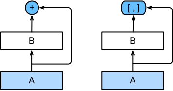
In the above figure, ResNet is on the left and DenseNet is on the right. Their main differences across layers are: using addition and using connection.
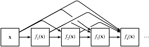
Therefore, after applying more and more complex function sequences, we perform from x \mathbf{x} Mapping of x to its expansion:
x → [ x , f 1 ( x ) , f 2 ( [ x , f 1 ( x ) ] ) , f 3 ( [ x , f 1 ( x ) , f 2 ( [ x , f 1 ( x ) ] ) ] ) , ... ] \mathbf{x} \rightarrow\left[\mathbf{x}, f_{1}(\mathbf{x}), f_{2}\left(\left[\mathbf{x}, f_{1}(\mathbf{x})\right]\right), f_{3}\left(\left[\mathbf{x}, f_{1}(\mathbf{x}), f_{2}\left(\left[\mathbf{x}, f_{1}(\mathbf{x})\right]\right)\right]\right), \ldots\right] x→[x,f1(x),f2([x,f1(x)]),f3([x,f1(x),f2([x,f1(x)])]),...]
Finally, these expansions are combined into multi-layer perceptron to reduce the number of features again. The implementation is very simple: we don't need to add terms, but connect them. The name DenseNet comes from the "dense connection" between variables, and the last layer is closely connected with all previous layers. Dense connection is shown in the figure below:
Dense network is mainly composed of two parts: dense block and transition block. The former defines how to connect inputs and outputs, while the latter controls the number of channels so that it is not too complex.
Dense block
DenseNet uses the improved "batch normalization, activation and convolution" structure of ResNet. Let's first implement this structure.
import torch
from torch import nn
from d2l import torch as d2l

def conv_block(input_channels, num_channels):
	return nn.Sequential(
		nn.BatchNorm2d(input_channels), nn.ReLU(),
		nn.Conv2d(input_channels, num_channels, kernel_size=3, padding=1)
	)
A dense block is composed of multiple convolution blocks, and each convolution block uses the output channel of the same vector. However, in forward propagation, we link the input and output of each convolution block in the channel dimension.
class DenseBlock(nn.Module):
	def __init__(self, num_convs, input_channels, num_channels):
		super(Denseblock, self).__init__()
		layer = []
		for i in range(num_convs):
			layer.append(conv_block(num_channels * i + input_channels, num_channels))
		self.net = nn.Sequential(*layer)

	def forward(self, X):
		for blk in self.net:
			Y = blk(X)
			# Connect the inputs and outputs of each block on the channel dimension
			X = torch.cat((X, Y), dim=1)
		return X
In the following example, we define a DenseBlock with two output channels of 10. When using an input with a channel number of 3, we will get a channel number of 3 + 2 × 10 = 23 3+2\times10=23 3+2 × 10 = 23 output. The number of channels of the convolution block controls the growth of the number of output channels relative to the number of input channels, so it is also called growth rate.
blk = DenseBlock(2, 3, 10)
X = torch.randn(4, 3, 8, 8)
Y = blk(X)
Y.shape
torch.Size([4, 23, 8, 8])
Transition layer
Because each dense fast will increase the number of channels, using too much will complicate the model too much. The transition layer can be used to control the complexity of the model. It passes 1 × 1 1\times1 one × 1 convolution layer to reduce the number of channels, and use the average convergence layer with step 2 to halve the height and width, so as to further reduce the complexity of the model.
def transition_block(input_channels, num_channels):
	return nn.Sequential(
		nn.BatchNorm2d(input_channels), nn.ReLU(),
		nn.Conv2d(input_channels, num_channels, kernel_size=1)
		nn.AvgPool2d(kernel_size=2, stride=2)
	)
For the output of dense blocks in the previous example, a transition layer with 10 channels is used. At this time, the number of output channels is reduced to 10, and the height and width are halved.
blk = transition_block(23, 10)
blk(Y).shape
torch.Size([4, 10, 4, 4])
DenseNet model
Let's construct the DenseNet model. DenseNet first uses the same single volume layer and maximum aggregation layer as ResNet.
b1 = nn.Sequential(
	nn.Conv2d(1, 64, kernel_size=7, stride=2, padding=3),
	nn.BatchNorm2d(64), nn.ReLU(),
	nn.MaxPool2d(kernel_size=3, stride=2, padding=1)
)
Next, similar to the four residual blocks used by ResNet, DenseNet uses four dense blocks. Similar to ResNet, we can set how many convolution layers each dense block uses. Here we set it to 4, which is consistent with the previous ResNet-18. The number of convolution layer channels (i.e. growth rate) in dense blocks is set to 32, so 128 channels will be added to each dense block.
Between each module, ResNet reduces the height and width through the residual block with step 2, while DenseNet uses the transition layer to halve the height and width and halve the number of channels.
# 'num_channels' is the current number of channels
num_channels, growth_rate = 64, 32
num_convs_in_dense_blocks = [4, 4, 4, 4]
blks = []
for i, num_convs in enumerate(num_convs_in_dense_blocks):
	blks.append(DenseBlock(num_convs, num_channels, growth_rate))
	# Number of output channels of the last dense block
	num_channels += num_convs * growth_rate
	# Add a transition layer between dense blocks to halve the number of channels
	if i != len(num_convs_in_dense_blocks) - 1:
		blks.append(transition_block(num_channels, num_channels // 2))
		num_channels = num_channels // 2
Similar to ResNet, the global aggregation layer and the full connection layer are connected to output the results.
net = nn.Sequential(
	b1, *blks,
	nn.BatchNorm2d(num_channels), nn.ReLU(),
	nn.AdaptiveMaxPool2d((1, 1)),
	nn.Flatten(),
	nn.Linear(num_channels, 10)
)
Training model
Since a deep network is used here, in this section, we reduce the input height and width from 224 to 96 to simplify the calculation.
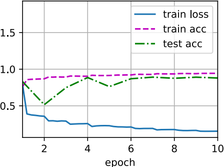
lr, num_epochs, batch_size = 0.1, 10, 256
train_iter, test_iter = d2l.load_data_fashion_mnist(batch_size, resize=96)
d2l.train_ch6(net, train_iter, test_iter, num_epochs, lr, d2l.try_gpu())
loss 0.154, train acc 0.943, test acc 0.880
5506.9 examples/sec on cuda:0