It is very difficult to train deep neural networks, especially in short practice. In this section, we will introduce batch normalization, which is a popular and effective technology to continuously accelerate the convergence speed of deep networks. After the combination, the residual will be introduced quickly, and batch normalization enables researchers to train networks with more than 100 layers.

Training deep network

Why batch normalization layer? Let's review some practical challenges in training neural networks:

1. The way of data preprocessing usually has a great impact on the final result. Recall our example of using multi-layer perceptron to predict house prices. When using real data, our first step is to standardize the input features so that the average value is 0 and the variance is 1. Intuitively, this standardization can be used well with our optimizer because it can unify the magnitude of parameters.
2. For a typical multilayer perceptron or convolution extended into the network. When we train, the variables in the middle layer (for example, affine transformation output in multi-layer perceptron) may have a wider range of variation: whether along the layer from input to output, across units in the same layer, or over time, the parameters of the model are unpredictable with the training update. The inventors of batch normalization informally assume that this offset in the distribution of these variables may hinder the convergence of the network. Intuitively, we may guess that if the variable value of one layer is 100 times that of another layer, it may need to compensate and adjust the learning rate.
3. Third, the deeper network is complex and easy to over fit. This means that regularization becomes more necessary.

Batch normalization is applied to a single optional layer (or to all layers), and its principle is as follows:
In each training iteration, we first normalize the input by subtracting its average and dividing it by its standard deviation, both of which are based on the current small batch processing.
Next, we apply a scale factor and a scale offset.
It is this standardization based on batch statistics that gives the name of batch standardization.

Here, if we try to apply small batch normalization with a small batch size of 1, we will not learn anything. This is because after subtracting the mean, each hidden cell will be 0. Therefore, batch normalization is effective and stable only when a large enough small batch is used. Note that when applying batch normalization, the selection of batch size may be more important than when there is no batch normalization.

Now let's look at how batch normalization works in practice.

Batch normalization layer

Recall that a key difference between batch normalization and other layers is that since batch normalization runs on complete small batches, we cannot ignore the size of batch processing when introducing other layers as before. We discuss these two cases below: full connection layer and convolution layer, and their batch normalization implementation is slightly different.

Full connection layer

Generally, we place the batch normalization layer between the affine transformation and the activation function in the full connection layer.

Convolution layer

Similarly, for convolution layer, we can apply batch normalization after convolution layer and before nonlinear activation function. When the convolution has multiple output channels, we need to perform batch normalization on the "each" output of these channels. Each user has its own stretch and offset parameters, both of which are scalars. Suppose our micro batch contains m m m examples, and for each channel, the output of the convolution has a height p p p and width q q q. So for the convolution layer, we're at the end of each output channel m ∗ p ∗ q m*p*q Each batch normalization is performed simultaneously on m * p * q elements. Therefore, when calculating the mean and variance, we collect the values of all spatial locations, and then apply the same mean and variance in a given channel to normalize the values at each spatial location.

Batch normalization in prediction process

As we mentioned earlier, batch normalization usually behaves differently in training mode and prediction mode.
Firstly, when the trained model is used for prediction, we no longer need the noise in the sample mean and the sample variance generated by each small batch on the micro batch.
Second, for example, we may need to use our model to predict sample by sample. A common method is to estimate the sample mean and variance of the whole training data set by moving average, and use them to obtain the determined output. It can be seen that, like dropout, the calculation results of batch normalization layer in training mode and prediction mode are also different.

LeNet using batch normalization layer

To better understand how to apply BatchNorm, let's apply it to the LeNet model. Recall that batch normalization is applied after the convolution layer or full connection layer and before the corresponding activation function.

net = nn.Sequential(
	nn.Conv2d(1, 6, kernel_size = 5), BatchNorm(6, num_dims=4), nn.Sigmoid(),
	nn.MaxPool2d(kernel_size=2, stride=2)
	nn.Conv2d(6, 16, kernel_size=5), BatchNorm(16, num_dims=4), nn.Sigmoid(),
	nn.MaxPool2d(kernel_size=2, stride=2), nn.Flatten(),
	nn.Linear(16*4*4, 120), BatchNorm(120, num_dims=2), nn.Sigmoid(),
	nn.Linear(120, 84), BatchNorm(84, num_dims=2), nn.Sigmoid(),
	nn.Linear(84, 10)
)

As before, we will train the network on the fashion MNIST dataset. This code is almost the same as when we first trained LeNet. The main difference is that the learning rate is much higher.

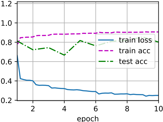
lr, num_epochs, batch_size = 1.0, 10, 256
train_iter, test_iter = d2l.load_data_fashion_mnist(batch_size)
d2l.train_ch6(net, train_iter, test_iter, num_epochs, lr, d2l.try_gpu())

loss 0.250, train acc 0.907, test acc 0.801
35560.7 examples/sec on cuda:0

Let's take a look at the stretching parameter gamma and the cheap parameter beta learned from the first batch normalization layer.

net[1].gamma.reshape((-1,)), net[1].beta.reshape((-1,))

(tensor([0.7562, 1.2784, 2.3527, 1.3189, 2.0457, 2.8424], device='cuda:0',
grad_fn=<ViewBackward>),
tensor([ 0.7436, -0.8156, -0.2711, -0.5087, 0.5847, -3.0033], device='cuda:0',
grad_fn=<ViewBackward>))

Concise implementation

In addition to using the BatchNorm we just defined, we can also directly use the BatchNorm defined in the deep learning framework. The code looks almost the same as our code above.

net = nn.Sequential(
nn.Conv2d(1, 6, kernel_size=5), nn.BatchNorm2d(6), nn.Sigmoid(),
nn.MaxPool2d(kernel_size=2, stride=2),
nn.Conv2d(6, 16, kernel_size=5), nn.BatchNorm2d(16), nn.Sigmoid(),
nn.MaxPool2d(kernel_size=2, stride=2), nn.Flatten(),
nn.Linear(256, 120), nn.BatchNorm1d(120), nn.Sigmoid(),
nn.Linear(120, 84), nn.BatchNorm1d(84), nn.Sigmoid(),
nn.Linear(84, 10))

Next, we use the same super parameters to train the model. Note that in general, the advanced API variant runs much faster because its code has been compiled into C + + or CUDA, and our custom code is implemented by Python.

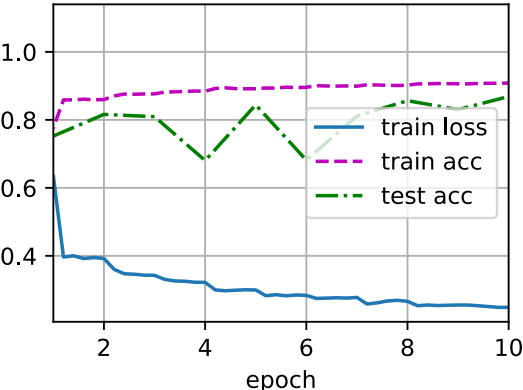
d2l.train_ch6(net, train_iter, test_iter, num_epochs, lr, d2l.try_gpu())

loss 0.248, train acc 0.908, test acc 0.869
60219.9 examples/sec on cuda:0

dispute

Intuitively, batch normalization is considered to make the optimization smoother.

However, in the paper of batch normalization, the author not only introduces its application, but also explains its principle: by reducing internal covariates. However, this explanation is more inclined to personal intuition.

However, the effect of batch normalization is very good. It is applicable to almost all image classifiers and has been cited by tens of thousands of scholars.