7 single shot multi frame detection (SSD)

The bounding box, anchor box, multi-scale target detection and data set for target detection are introduced respectively. Now we are ready to use this background knowledge to design a target detection model: single shot multibox detector (SSD).

7.1 model

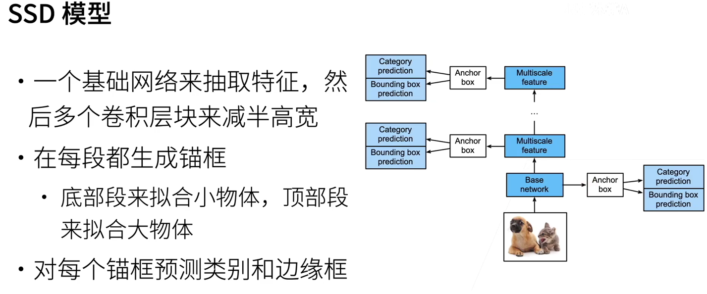
This model is mainly composed of basic network, followed by several multi-scale feature blocks. The basic network is used to extract features from the input image, so it can use deep convolution neural network. We can design the basic network to make its output higher and wider. In this way, the number of anchor frames generated based on the feature map is large, which can be used to detect smaller targets. Next, each multi-scale feature block reduces the height and width of the feature map provided by the previous layer (e.g. halving), and makes the receptive field of each unit in the feature map on the input image wider. It can be used to detect large targets.

7.1.1 category prediction layer

Set the number of target categories as q. In this way, the anchor box has q+1 categories, of which category 0 is the background. If we generate a anchor box centered on each cell, we need to classify hwa anchor boxes. If the full connection layer is used as the output, it is easy to lead to too many model parameters.
Consider outputting and inputting the same spatial coordinates (x, y): the channel of (x, y) coordinates on the output feature map contains the category prediction of all anchor boxes generated centered on the (x, y) coordinates of the input feature map. Therefore, the number of output channels is a(q+1), in which the channel with index i(q+1)+j (0 ≤ j ≤ q) represents the prediction of anchor box with index i and related category index j.

def cls_predictor(num_inputs, num_anchors, num_classes):
    return nn.Conv2d(num_inputs, num_anchors * (num_classes + 1),
                     kernel_size=3, padding=1)

7.1.2 boundary box prediction layer

The design of the bounding box prediction layer is similar to that of the category prediction layer. The only difference is that you need to predict 4 offsets for each anchor box instead of q+1 categories.

def bbox_predictor(num_inputs, num_anchors):
    return nn.Conv2d(num_inputs, num_anchors * 4, kernel_size=3, padding=1)

7.1.3 connecting MULTI-SCALE PREDICTION

As we mentioned, single shot multi frame detection uses multi-scale feature maps to generate anchor frames and predict their categories and offsets. At different scales, the shape of the feature map or the number of anchor frames centered on the same unit may be different. Therefore, the shape of prediction output may be different at different scales.

#   5 and 3 anchor boxes, assuming that the number of target categories is 10 
Y1 = forward(torch.zeros((2, 8, 20, 20)), cls_predictor(8, 5, 10))
Y2 = forward(torch.zeros((2, 16, 10, 10)), cls_predictor(16, 3, 10))
print(Y1.shape, Y2.shape)
################
torch.Size([2, 55, 20, 20]) torch.Size([2, 33, 10, 10])

In addition to the dimension of batch size, the other three dimensions have different sizes. In order to link the two prediction outputs to improve computational efficiency, we will convert these tensors into a more consistent format.

The channel dimension contains the prediction results of anchor boxes with the same center. We first move the channel dimension to the last dimension. Because the batch size remains unchanged at different scales, we can convert the prediction results into two-dimensional (batch size, high) × Wide × Number of channels) to facilitate subsequent links on dimension 1.

def flatten_pred(pred):
    return torch.flatten(pred.permute(0, 2, 3, 1), start_dim=1)

def concat_preds(preds):
    return torch.cat([flatten_pred(p) for p in preds], dim=1)

print(concat_preds([Y1, Y2]).shape)
#############
(2, 25300)

7.1.4 height and width halved

Each height and width halved block consists of two 3 filled with 1 × The convolution layer of 3 and 2 with a step of 2 × 2. Composition of maximum convergence layer. We know that 3 filled with 1 × The convolution layer does not change the shape of the characteristic graph. However, the following 2 × The maximum convergence layer of 2 reduces the height and width of the input feature map by half.

def down_sample_blk(in_channels, out_channels):
    blk = []
    for _ in range(2):
        blk.append(nn.Conv2d(in_channels, out_channels,
                             kernel_size=3, padding=1))
        blk.append(nn.BatchNorm2d(out_channels))
        blk.append(nn.ReLU())
        in_channels = out_channels
    blk.append(nn.MaxPool2d(2))
    return nn.Sequential(*blk)


print(forward(torch.zeros((2, 3, 20, 20)), down_sample_blk(3, 10)).shape)

7.1.5 basic network block

The basic network block is used to extract features from the input image. In order to simplify the calculation, we construct a small basic network, which connects three height and width halved blocks in series, and gradually doubles the number of channels.

def base_net():
    blk = []
    num_filters = [3, 16, 32, 64]
    for i in range(len(num_filters) - 1):
        blk.append(down_sample_blk(num_filters[i], num_filters[i+1]))
    return nn.Sequential(*blk)

print(forward(torch.zeros((2, 3, 256, 256)), base_net()).shape)
###############
torch.Size([2, 64, 32, 32])

7.1.6 complete model

The complete single shot multi frame detection model consists of five modules. The feature map generated by each block is used not only to (i) generate anchor boxes, but also to (ii) predict the category and offset of these anchor boxes. Among the five modules, the first is the basic network block, the second to the fourth is the height and width halved block, and the last module uses the global maximum pool to reduce the height and width to 1.

def get_blk(i):
    if i == 0:
        blk = base_net()
    elif i == 1:
        blk = down_sample_blk(64, 128)
    elif i == 4:
        blk = nn.AdaptiveMaxPool2d((1,1))
    else:
        blk = down_sample_blk(128, 128)
    return blk

Now we define a forward calculation for each block. Unlike the image classification task, the output here includes: (i) CNN feature map Y, (ii) anchor frames generated according to Y at the current scale, and (iii) predicted categories and offsets of these anchor frames (based on Y).

def blk_forward(X, blk, size, ratio, cls_predictor, bbox_predictor):
    Y = blk(X)
    anchors = d2l.multibox_prior(Y, sizes=size, ratios=ratio)
    cls_preds = cls_predictor(Y)
    bbox_preds = bbox_predictor(Y)
    return (Y, anchors, cls_preds, bbox_preds)

A multi-scale feature block close to the top is used to detect larger targets, so it is necessary to generate larger anchor boxes. In the above forward calculation, on each multi-scale feature block, we call the multibox_ The sizes parameter of the prior function passes a list of two proportional values.

sizes = [[0.2, 0.272], [0.37, 0.447], [0.54, 0.619], [0.71, 0.79],
         [0.88, 0.961]]
ratios = [[1, 2, 0.5]] * 5
num_anchors = len(sizes[0]) + len(ratios[0]) - 1

class TinySSD(nn.Module):
    def __init__(self, num_classes, **kwargs):
        super(TinySSD, self).__init__(**kwargs)
        self.num_classes = num_classes
        idx_to_in_channels = [64, 128, 128, 128, 128]
        for i in range(5):
            # Assignment statement ` self.blk_i = get_blk(i)`
            setattr(self, f'blk_{i}', get_blk(i))
            setattr(self, f'cls_{i}', cls_predictor(idx_to_in_channels[i],
                                                    num_anchors, num_classes))
            setattr(self, f'bbox_{i}', bbox_predictor(idx_to_in_channels[i],
                                                      num_anchors))

    def forward(self, X):
        anchors, cls_preds, bbox_preds = [None] * 5, [None] * 5, [None] * 5
        for i in range(5):
            # `Getattr (self, 'blk_%d'% I) ` access ` self.blk_i`
            X, anchors[i], cls_preds[i], bbox_preds[i] = blk_forward(
                X, getattr(self, f'blk_{i}'), sizes[i], ratios[i],
                getattr(self, f'cls_{i}'), getattr(self, f'bbox_{i}'))
        anchors = torch.cat(anchors, dim=1)
        cls_preds = concat_preds(cls_preds)
        cls_preds = cls_preds.reshape(
            cls_preds.shape[0], -1, self.num_classes + 1)
        bbox_preds = concat_preds(bbox_preds)
        return anchors, cls_preds, bbox_preds

net = TinySSD(num_classes=1)
X = torch.zeros((32, 3, 256, 256))
anchors, cls_preds, bbox_preds = net(X)

print('output anchors:', anchors.shape)
print('output class preds:', cls_preds.shape)
print('output bbox preds:', bbox_preds.shape)
#################
output anchors: torch.Size([1, 5444, 4])
output class preds: torch.Size([32, 5444, 2])
output bbox preds: torch.Size([32, 21776])

7.2 training model

7.2.1 read data set and initialization

In banana detection dataset, the number of target categories is 1. After defining the model, we need to initialize its parameters and define the optimization algorithm.

batch_size = 32
train_iter, _ = d2l.load_data_bananas(batch_size)

device, net = d2l.try_gpu(), TinySSD(num_classes=1)
trainer = torch.optim.SGD(net.parameters(), lr=0.2, weight_decay=5e-4)

7.2.2 define loss function and evaluation function

There are two types of losses in target detection. The first is about the loss of anchor box category: we can simply reuse the cross entropy loss function used in image classification problems before; The second is about the loss of positive anchor box offset: the predicted offset is a regression problem. However, for this regression problem, we do not use the square loss described in, but use the L1 norm loss, that is, the absolute value of the difference between the predicted value and the real value. Mask variable bbox_masks makes the negative anchor frame and filled anchor frame not participate in the loss calculation. Finally, we add the loss of anchor box category and offset to obtain the final loss function of the model.

cls_loss = nn.CrossEntropyLoss(reduction='none')
bbox_loss = nn.L1Loss(reduction='none')

def calc_loss(cls_preds, cls_labels, bbox_preds, bbox_labels, bbox_masks):
    batch_size, num_classes = cls_preds.shape[0], cls_preds.shape[2]
    cls = cls_loss(cls_preds.reshape(-1, num_classes),
                   cls_labels.reshape(-1)).reshape(batch_size, -1).mean(dim=1)
    bbox = bbox_loss(bbox_preds * bbox_masks,
                     bbox_labels * bbox_masks).mean(dim=1)
    return cls + bbox

We can use the accuracy rate to evaluate the classification results. Since the L1 norm loss is used in the offset, we use the average absolute error to evaluate the prediction results of the bounding box. These prediction results are obtained from the generated anchor box and its prediction offset.

def cls_eval(cls_preds, cls_labels):
    # Because the category prediction result is placed in the last dimension, 'argmax' needs to specify the last dimension.
    return float((cls_preds.argmax(dim=-1).type(
        cls_labels.dtype) == cls_labels).sum())

def bbox_eval(bbox_preds, bbox_labels, bbox_masks):
    return float((torch.abs((bbox_labels - bbox_preds) * bbox_masks)).sum())

7.2.3 training model

num_epochs, timer = 20, d2l.Timer()
animator = d2l.Animator(xlabel='epoch', xlim=[1, num_epochs],
                        legend=['class error', 'bbox mae'])
net = net.to(device)
for epoch in range(num_epochs):
    # Sum of training accuracy, number of examples in the sum of training accuracy
    # Sum of absolute errors, number of examples in the sum of absolute errors
    metric = d2l.Accumulator(4)
    net.train()
    for features, target in train_iter:
        timer.start()
        trainer.zero_grad()
        X, Y = features.to(device), target.to(device)
        # Generate multi-scale anchor boxes and predict categories and offsets for each anchor box
        anchors, cls_preds, bbox_preds = net(X)
        # Label the category and offset for each anchor box
        bbox_labels, bbox_masks, cls_labels = d2l.multibox_target(anchors, Y)
        # Calculate the loss function based on the predicted and labeled values of category and offset
        l = calc_loss(cls_preds, cls_labels, bbox_preds, bbox_labels,
                      bbox_masks)
        l.mean().backward()
        trainer.step()
        metric.add(cls_eval(cls_preds, cls_labels), cls_labels.numel(),
                   bbox_eval(bbox_preds, bbox_labels, bbox_masks),
                   bbox_labels.numel())
    cls_err, bbox_mae = 1 - metric[0] / metric[1], metric[2] / metric[3]
    animator.add(epoch + 1, (cls_err, bbox_mae))
print(f'class err {cls_err:.2e}, bbox mae {bbox_mae:.2e}')
print(f'{len(train_iter.dataset) / timer.stop():.1f} examples/sec on '
      f'{str(device)}')
      
plt.show()

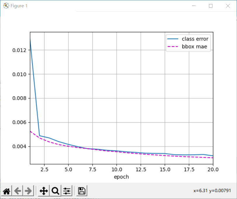
class err 3.21e-03, bbox mae 3.04e-03
1110.2 examples/sec on cpu

8 regional convolutional neural network (R-CNN) series

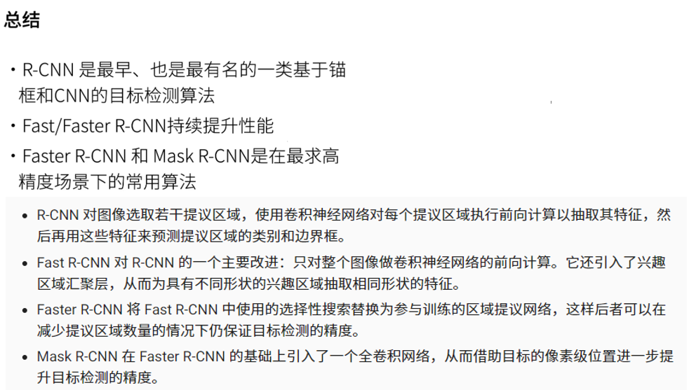
In addition to single shot multi frame detection, regional convolutional neural network (region based CNN or regions with CNN features, R-CNN) is also one of the pioneering work of applying depth model to target detection. In this section, we will introduce R-CNN and a series of improvement methods: Fast R-CNN, Faster R-CNN and Mask R-CNN.

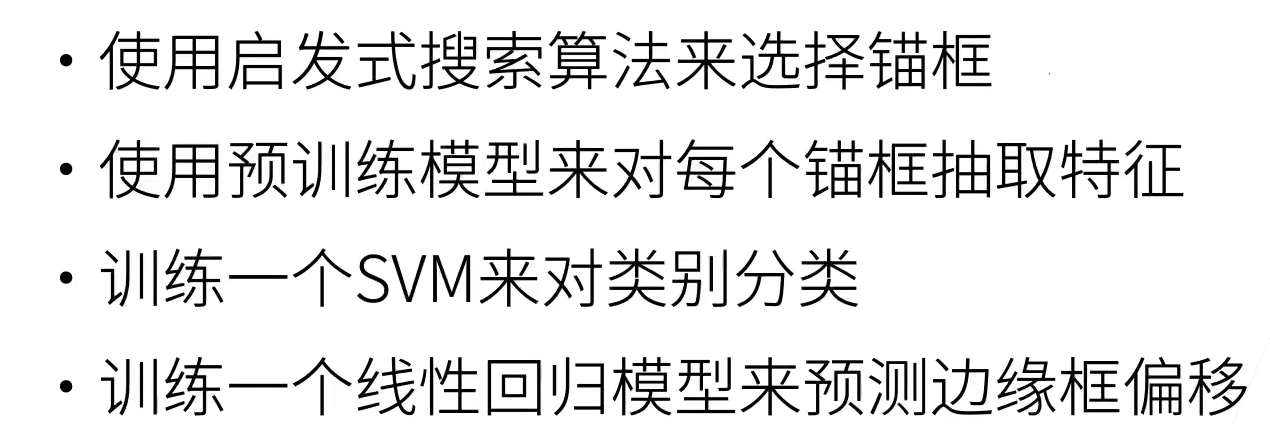
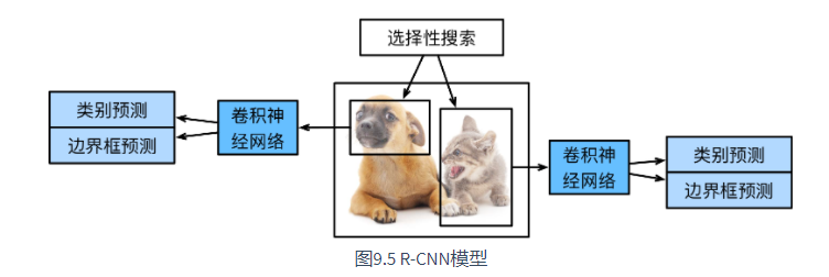
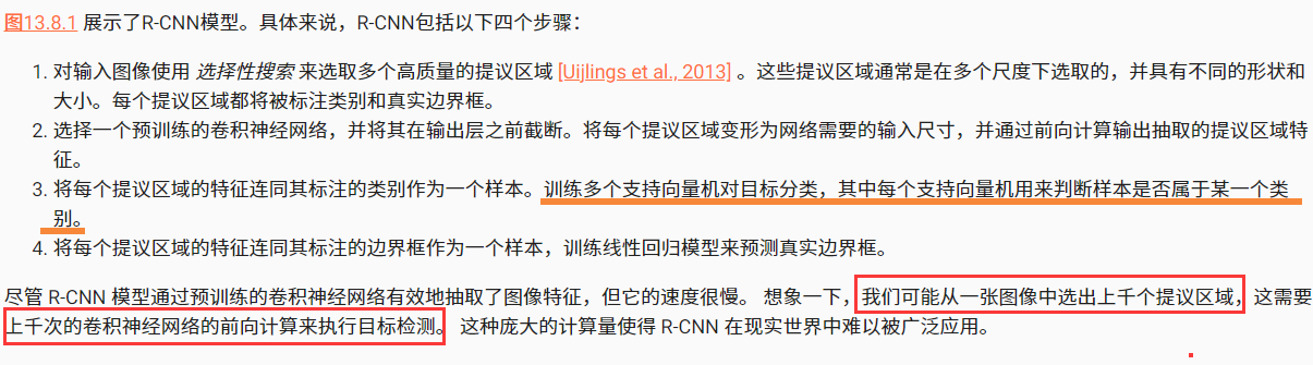
8.1 R-CNN

R-CNN first selects several proposed areas (e.g. 2000) from the input image (e.g. anchor box is also a selection method), and labels their categories and bounding boxes (e.g. offset). Then, the convolution neural network is used to calculate the forward of each proposed region to extract its features. Next, we use the characteristics of each proposed area to predict the category and bounding box.

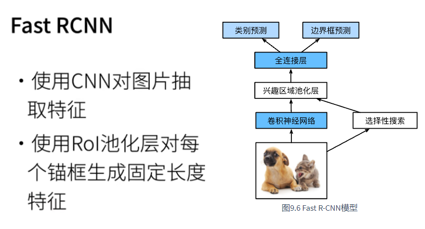
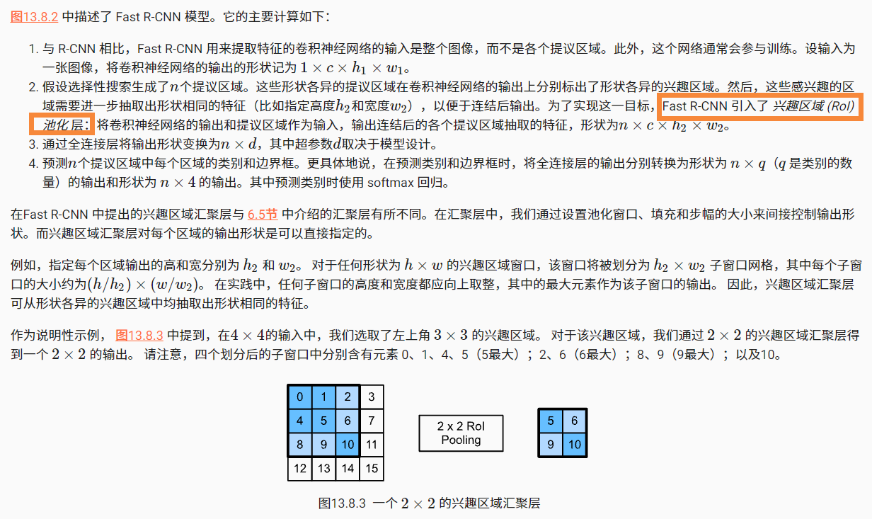
8.2 Fast R-CNN

The main performance bottleneck of R-CNN is that for each proposed region, the forward calculation of convolutional neural network is independent without shared calculation. Because these regions usually overlap, independent feature extraction will lead to repeated calculations. One of the main improvements of Fast R-CNN [Girshick, 2015] to R-CNN is to perform forward calculation of convolutional neural network only on the whole image.

import torch
import torchvision

X = torch.arange(16.).reshape(1, 1, 4, 4)
rois = torch.Tensor([[0, 0, 0, 20, 20], [0, 0, 10, 30, 30]])
print(torchvision.ops.roi_pool(X, rois, output_size=(2, 2), spatial_scale=0.1))
#################
tensor([[[[ 5.,  6.],
          [ 9., 10.]]],
        [[[ 9., 11.],
          [13., 15.]]]])

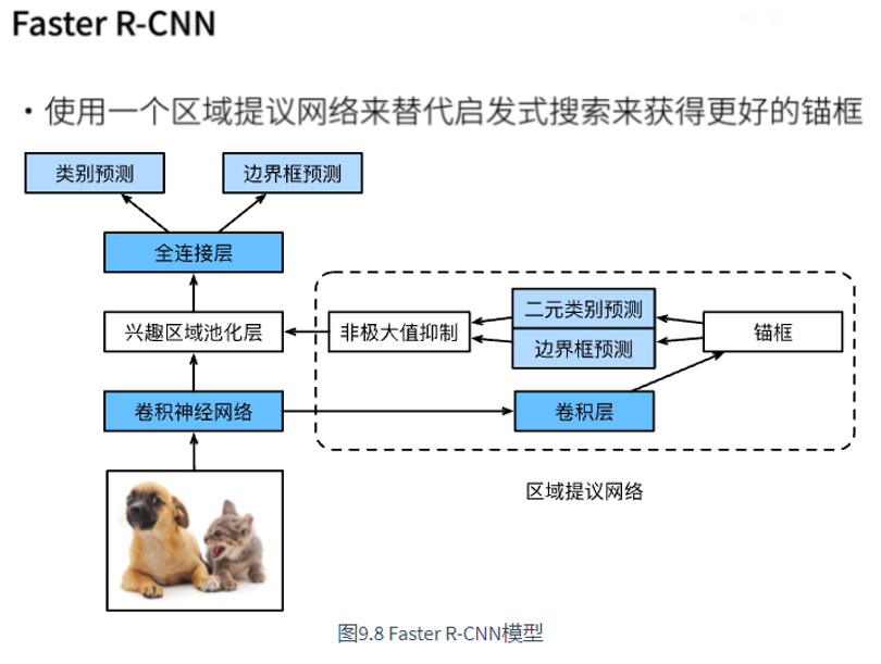
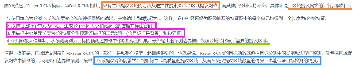
8.3 Faster R-CNN

Fast R-CNN usually needs to generate more proposed areas in selective search to obtain more accurate target detection results. Fast R-CNN proposes to replace selective search with regional proposal network, so as to reduce the number of proposed areas and ensure the accuracy of target detection.

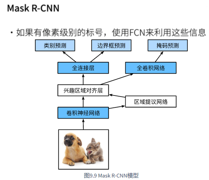
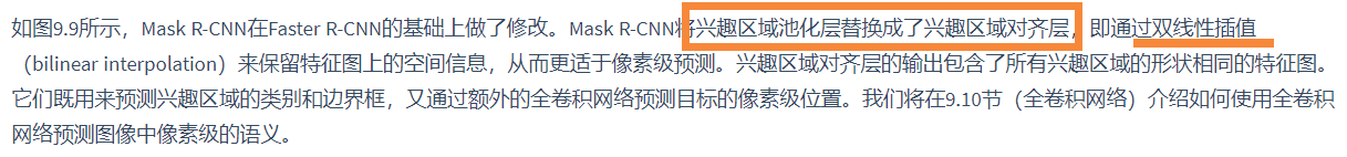
8.4 Mask R-CNN

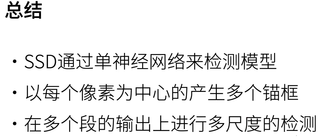
8.5 summary

9 semantic segmentation and dataset

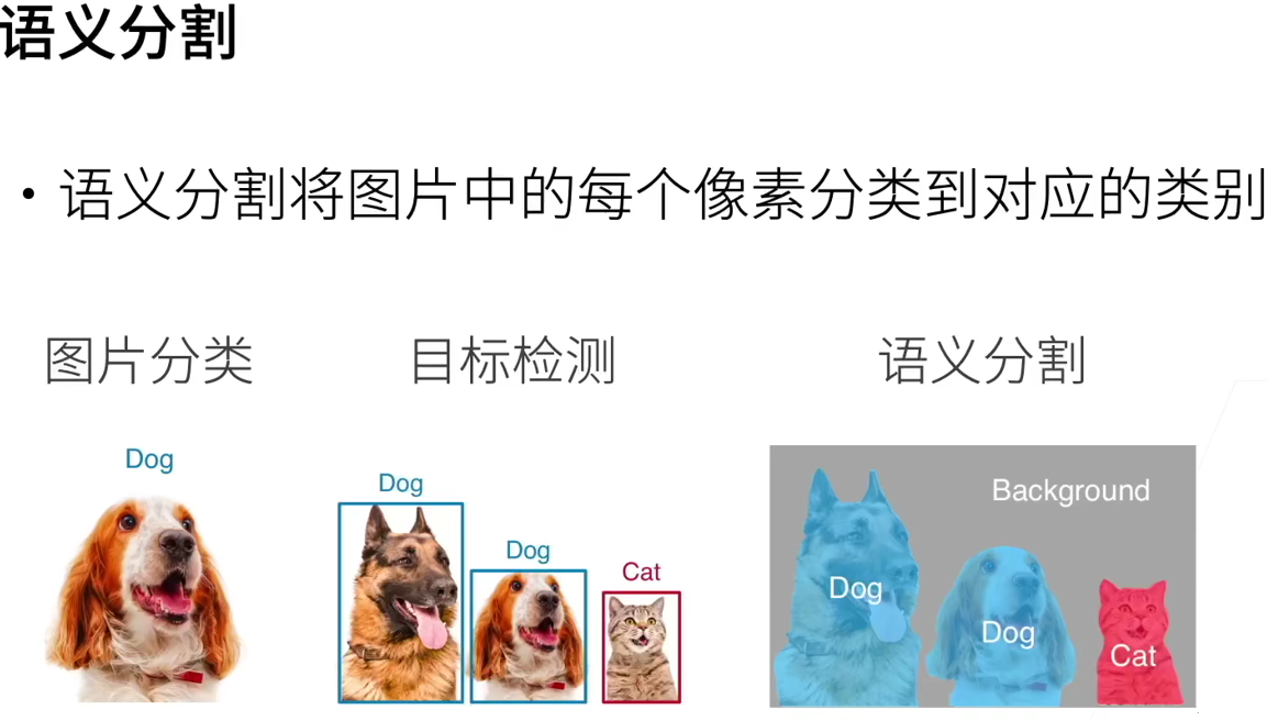
Semantic segmentation focuses on how to segment an image into regions belonging to different semantic categories. Different from target detection, semantic segmentation can recognize and understand the content of each pixel in the image: the annotation and prediction of its semantic region are pixel level. Compared with target detection, the pixel level frame of semantic segmentation annotation is obviously more fine.

9.1 image segmentation and instance segmentation

There are also two important problems similar to semantic segmentation in the field of computer vision, namely image segmentation and instance segmentation. Here we briefly distinguish them from semantic segmentation.

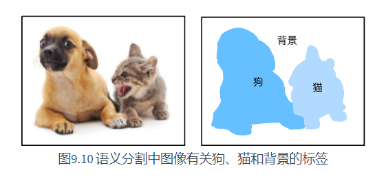
• Image segmentation divides the image into several constituent regions. The methods of this kind of problem usually use the correlation between pixels in the image. It does not need label information about image pixels in training, and it can not guarantee that the segmented region has the semantics we want in prediction. Taking the image in Figure 9.10 as the input, image segmentation may divide the dog into two areas: one covers the mouth and eyes dominated by black, and the other covers the rest of the body dominated by yellow.
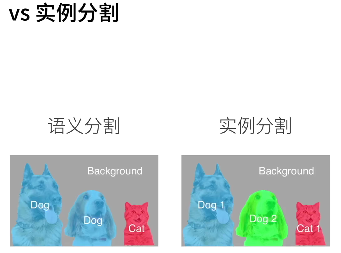
• Instance segmentation is also called simultaneous detection and segmentation. It studies how to identify the pixel level region of each target instance in the image. Unlike semantic segmentation, instance segmentation needs to distinguish not only semantics, but also different target instances. For example, if there are two dogs in the image, the instance segmentation needs to distinguish which of the two dogs the pixel belongs to.

9.2 Pascal VOC2012 semantic segmentation dataset

The tar file of the dataset is about 2GB, so the download may take some time.

d2l.DATA_HUB['voc2012'] = (d2l.DATA_URL + 'VOCtrainval_11-May-2012.tar',
                           '4e443f8a2eca6b1dac8a6c57641b67dd40621a49')

voc_dir = d2l.download_extract('voc2012', 'VOCdevkit/VOC2012')

def read_voc_images(voc_dir, is_train=True):
    txt_fname = os.path.join(voc_dir, 'ImageSets', 'Segmentation',
                             'train.txt' if is_train else 'val_txt')
    mode = torchvision.io.image.ImageReadMode.RGB
    with open(txt_fname, 'r') as f:
        images = f.read().split()
    features, labels = [], []
    for i, fname in enumerate(images):
        features.append(torchvision.io.read_image(os.path.jion(
            voc_dir, 'JPEGImages', f'{fname}.jpg')))
        labels.append(torchvision.io.read_image(os.path.join(
            voc_dir, 'SegmentationClass', f'{fname}.png'), mode))
    return features, labels


train_features, train_labels = read_voc_images(voc_dir, True)

n = 5
imgs = train_features[0:n] + train_labels[0:n]
imgs = [img.permute(1,2,0) for img in imgs]
d2l.show_images(imgs, 2, n)
plt.show()

enumerate function record

If you want to traverse both indexes and elements for a list, you can write this:

for index, item in enumerate(list1):
    print index, item

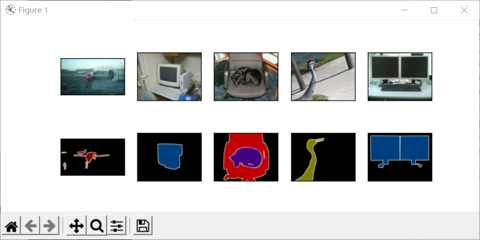
Next, we list RGB color values and class names.

#@save
VOC_COLORMAP = [[0, 0, 0], [128, 0, 0], [0, 128, 0], [128, 128, 0],
                [0, 0, 128], [128, 0, 128], [0, 128, 128], [128, 128, 128],
                [64, 0, 0], [192, 0, 0], [64, 128, 0], [192, 128, 0],
                [64, 0, 128], [192, 0, 128], [64, 128, 128], [192, 128, 128],
                [0, 64, 0], [128, 64, 0], [0, 192, 0], [128, 192, 0],
                [0, 64, 128]]

VOC_CLASSES = ['background', 'aeroplane', 'bicycle', 'bird', 'boat',
               'bottle', 'bus', 'car', 'cat', 'chair', 'cow',
               'diningtable', 'dog', 'horse', 'motorbike', 'person',
               'potted plant', 'sheep', 'sofa', 'train', 'tv/monitor']

Through the two constants defined above, we can easily find the class index of each pixel in the label.

def voc_colormap2label():
    colormap2label = torch.zeros(256 ** 3, dtype=torch.long)
    for i, colormap in enumerate(VOC_COLORMAP):
        colormap2label[
            (colormap[0] * 256 + colormap[1]) * 256 + colormap[2]] = i
    return colormap2label


def voc_label_indices(colormap, colormap2label):
    colormap = colormap.permute(1, 2, 0).numpy().astype('int32')
    idx = ((colormap[:, :, 0] * 256 + colormap[:, :, 1]) * 256
           + colormap[:, :, 2])
    return colormap2label[idx]

We define VOC_ The colormap2label function is used to build the mapping from the above RGB color value to the category index, while VOC_ label_ The indexes function maps RGB values to category indexes in the Pascal VOC2012 dataset.

9.2.1 preprocessing data

In previous experiments, we scaled the image to fit the input shape of the model. However, in semantic segmentation, this requires remapping the predicted pixel categories back to the original size of the input image. Such mapping may not be accurate enough, especially in segmented regions with different semantics. To avoid this problem, we crop the image to a fixed size instead of scaling. Specifically, we use random clipping in image augmentation to clip the same area of the input image and the label.

def voc_rand_crop(feature, label, height, width):
    rect = torchvision.transforms.RandomCrop.get_params(
        feature, (height, width))
    feature = torchvision.transforms.functional.crop(feature, *rect)
    label = torchvision.transforms.functional.crop(label, *rect)
    return feature, label

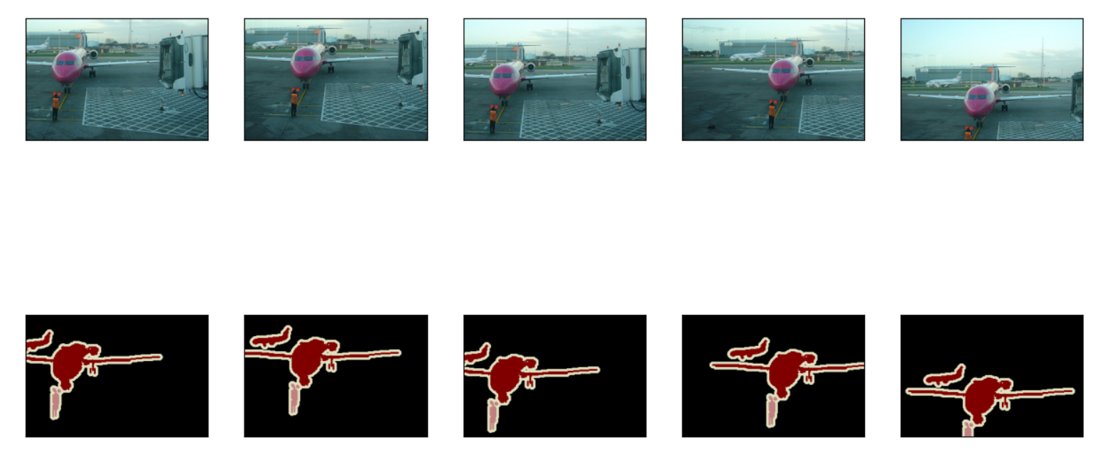
imgs = []
for _ in range(n):
    imgs += voc_rand_crop(train_features[0], train_labels[0], 200, 300)

imgs = [img.permute(1, 2, 0) for img in imgs]
d2l.show_images(imgs[::2] + imgs[1::2], 2, n)
plt.show()

9.2.2 custom semantic segmentation dataset class

By inheriting the Dataset class provided by the advanced API, a semantic segmentation Dataset class VOCSegDataset is customized. By implementing_ getitem _ _ Function, we can arbitrarily access the input image indexed as idx in the Dataset and the category index of each pixel. Since the size of some images in the Dataset may be smaller than the output size specified by random clipping, these samples can be removed through the custom filter function. In addition, we define normalize_image function to standardize the values of the three RGB channels of the input image.

#@save
class VOCSegDataset(torch.utils.data.Dataset):
    def __init__(self, is_train, crop_size, voc_dir):
        self.transform = torchvision.transforms.Normalize(
            mean=[0.485, 0.456, 0.406], std=[0.229, 0.224, 0.225])
        self.crop_size = crop_size
        features, labels = read_voc_images(voc_dir, is_train=is_train)
        self.features = [self.normalize_image(feature)
                         for feature in self.filter(features)]
        self.labels = self.filter(labels)
        self.colormap2label = voc_colormap2label()
        print('read ' + str(len(self.features)) + ' examples')

    def normalize_image(self, img):
        return self.transform(img.float())

    def filter(self, imgs):
        return [img for img in imgs if (
            img.shape[1] >= self.crop_size[0] and
            img.shape[2] >= self.crop_size[1])]

    def __getitem__(self, idx):
        feature, label = voc_rand_crop(self.features[idx], self.labels[idx],
                                       *self.crop_size)
        return (feature, voc_label_indices(label, self.colormap2label))

    def __len__(self):
        return len(self.features)

9.2.3 reading data sets

Create instances of training set and test set respectively through the customized VOCSegDataset class. Suppose we specify that the shape of the randomly cropped output image is 320 × 480. Next, we can view the number of samples reserved in the training set and the test set.

crop_size = (320, 480)
voc_train = VOCSegDataset(True, crop_size, voc_dir)
voc_test = VOCSegDataset(False, crop_size, voc_dir)
###############
read 1114 examples
read 1078 examples

Let the batch size be 64, and we define the iterator of the training set. Printing the first small batch of shapes will find that, unlike image classification or target detection, the label here is a three-dimensional array.

batch_size = 64
train_iter = torch.utils.data.DataLoader(voc_train, batch_size, shuffle=True,
                                    drop_last=True,
                                    num_workers=d2l.get_dataloader_workers())
for X, Y in train_iter:
    print(X.shape)
    print(Y.shape)
    break
###########
torch.Size([64, 3, 320, 480])
torch.Size([64, 320, 480])

9.2.4 integration of all components

Finally, we define the following_ data_ VOC function to download and read Pascal VOC2012 semantic segmentation dataset. It returns data iterators for training sets and test sets.

#@save
def load_data_voc(batch_size, crop_size):
    """load VOC Semantic segmentation dataset."""
    voc_dir = d2l.download_extract('voc2012', os.path.join(
        'VOCdevkit', 'VOC2012'))
    num_workers = d2l.get_dataloader_workers()
    train_iter = torch.utils.data.DataLoader(
        VOCSegDataset(True, crop_size, voc_dir), batch_size,
        shuffle=True, drop_last=True, num_workers=num_workers)
    test_iter = torch.utils.data.DataLoader(
        VOCSegDataset(False, crop_size, voc_dir), batch_size,
        drop_last=True, num_workers=num_workers)
    return train_iter, test_iter

9.3 summary

• Semantic segmentation identifies and understands the pixel level content in the image by dividing the image into regions belonging to different semantic categories.
• An important data set for semantic segmentation is called Pascal VOC2012.
• Because the input image and label of semantic segmentation correspond one-to-one in pixels, the input image will be randomly cropped to a fixed size instead of scaling.

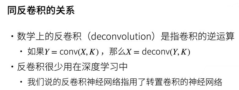
10 transpose convolution

So far, convolutional neural network layers, such as convolution layer and convergence layer, usually reduce the spatial dimensions (height and width) of down sampled input images. However, if the spatial dimensions of the input and output images are the same, it will be very convenient in the semantic segmentation of pixel level classification. For example, the channel dimension of the output pixel can retain the classification results of the input pixel at the same position.

In order to achieve this, especially after the spatial dimension is reduced by the convolution neural network layer, we can use another type of convolution neural network layer, which can increase the spatial dimension of the upper sampling middle layer feature map. In this section, we will introduce transposed convolution, which is used to reverse the spatial size reduction caused by down sampling.

10.1 basic operation

def trans_conv(X, K):
    h, w = K.shape
    Y = torch.zeros((X.shape[0] + h - 1, X.shape[1] + w - 1))
    for i in range(X.shape[0]):
        for j in range(X.shape[1]):
            Y[i: i + h, j: j + w] += X[i, j] * K
    return Y

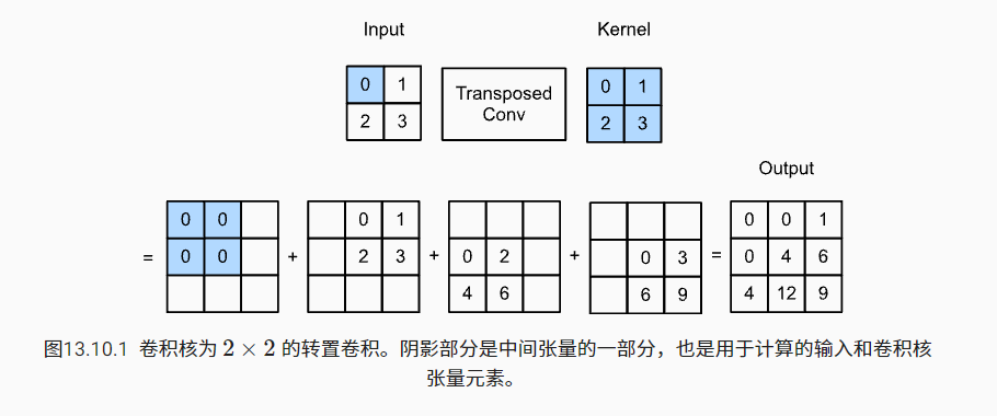
Compared with the conventional convolution of "reducing" the input elements through the convolution kernel, the transposed convolution "broadcasts" the input elements through the convolution kernel, resulting in an output larger than the input.

X = torch.tensor([[0.0, 1.0], [2.0, 3.0]])
K = torch.tensor([[0.0, 1.0], [2.0, 3.0]])
print(trans_conv(X, K))
###########################
tensor([[ 0.,  0.,  1.],
        [ 0.,  4.,  6.],
        [ 4., 12.,  9.]])

The same results can be obtained using the advanced API.

X, K = X.reshape(1, 1, 2, 2), K.reshape(1, 1, 2, 2)
tconv = nn.ConvTranspose2d(1, 1, kernel_size=2, bias=False)
tconv.weight.data = K
print(tconv(X))
#####################
tensor([[[[ 0.,  0.,  1.],
          [ 0.,  4.,  6.],
          [ 4., 12.,  9.]]]], grad_fn=<SlowConvTranspose2DBackward>)

nn.ConvTranspose2d function record

torch.nn.ConvTranspose2d(in_channels, out_channels, kernel_size, stride=1, padding=0, output_padding=0, bias=True)

10.2 filling, stride and multichannel

In transpose convolution, padding is applied to the output (conventional convolution applies padding to the input). For example, when the number of fills on both sides of height and width is specified as 1, the first and last rows and columns will be deleted in the output of transpose convolution.

tconv = nn.ConvTranspose2d(1, 1, kernel_size=2, padding=1, bias=False)
tconv.weight.data = K
print(tconv(X))
##########################
tensor([[[[4.]]]], grad_fn=<SlowConvTranspose2DBackward>)

In transpose convolution, the stride is specified as an intermediate result (output) rather than an input. Using the same input and convolution kernel tensor in figure 13.10.1, changing the stride from 1 to 2 will increase the height and weight of the intermediate tensor, so the output tensor is shown in figure 13.10.2.

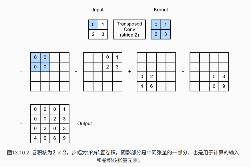
tconv = nn.ConvTranspose2d(1, 1, kernel_size=2, stride=2, bias=False)
tconv.weight.data = K
print(tconv(X))
###############################
tensor([[[[0., 0., 0., 1.],
          [0., 0., 2., 3.],
          [0., 2., 0., 3.],
          [4., 6., 6., 9.]]]], grad_fn=<SlowConvTranspose2DBackward>)

Substitute x into convolution layer f to output Y=f(X), and create a transposed convolution layer g with the same super parameters as F, but the number of output channels is the number of channels in X, then the shape of g(Y) will be the same as X.

X = torch.rand(size=(1, 10, 16, 16))
conv = nn.Conv2d(10, 20, kernel_size=5, padding=2, stride=3)
tconv = nn.ConvTranspose2d(20, 10, kernel_size=5, padding=2, stride=3)
print(tconv(conv(X)).shape == X.shape)
#########
True

10.3 connection with matrix transformation

We define a 3 × Inputs X and 2 for 3 × 2 convolution kernel K, and then use the corr2d function to calculate the convolution output Y.

X = torch.arange(9.0).reshape(3, 3)
K = torch.tensor([[1.0, 2.0], [3.0, 4.0]])
Y = d2l.corr2d(X, K)
######################
tensor([[27., 37.],
        [57., 67.]])

We rewrite the convolution kernel K into a sparse weight matrix W containing a large number of zeros. The shape of the weight matrix is (4, 9), where the non-0 element comes from the convolution kernel K.

def kernel2matrix(K):
    k, W = torch.zeros(5), torch.zeros((4, 9))
    k[:2], k[3:5] = K[0, :], K[1, :]
    W[0, :5], W[1, 1:6], W[2, 3:8], W[3, 4:] = k, k, k, k
    return W

W = kernel2matrix(K)
print(W)
###################
tensor([[1., 2., 0., 3., 4., 0., 0., 0., 0.],
        [0., 1., 2., 0., 3., 4., 0., 0., 0.],
        [0., 0., 0., 1., 2., 0., 3., 4., 0.],
        [0., 0., 0., 0., 1., 2., 0., 3., 4.]])

print(Y == torch.matmul(W, X.reshape(-1)).reshape(2, 2))
Z = trans_conv(Y, K)
Z = trans_conv(Y, K)
print(Z == torch.matmul(W.T, Y.reshape(-1)).reshape(3, 3))
################
tensor([[True, True],
        [True, True]])
tensor([[True, True, True],
        [True, True, True],
        [True, True, True]])

10.4 intuitive understanding of function parameter setting

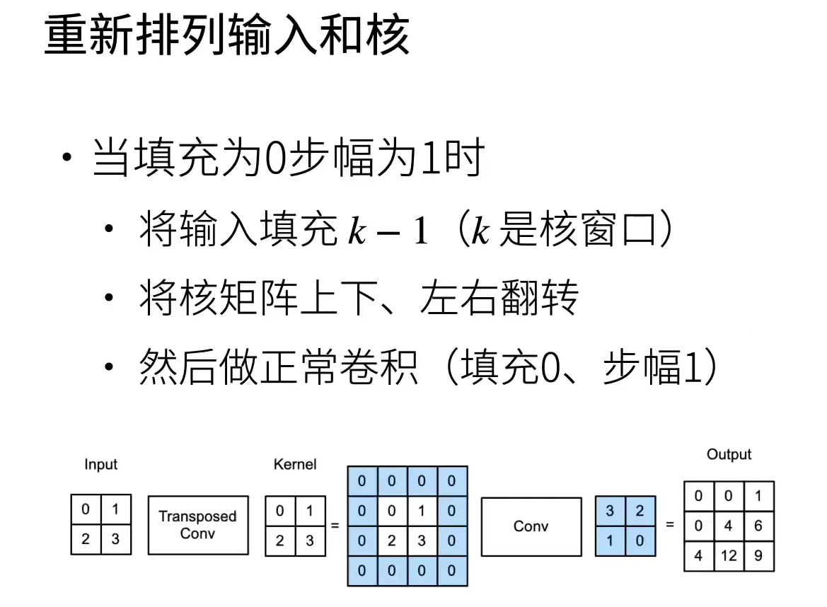
Fill the input with 2-1 layers, turn the kernel matrix left and right, up and down, and convolute to transpose the convolution value.

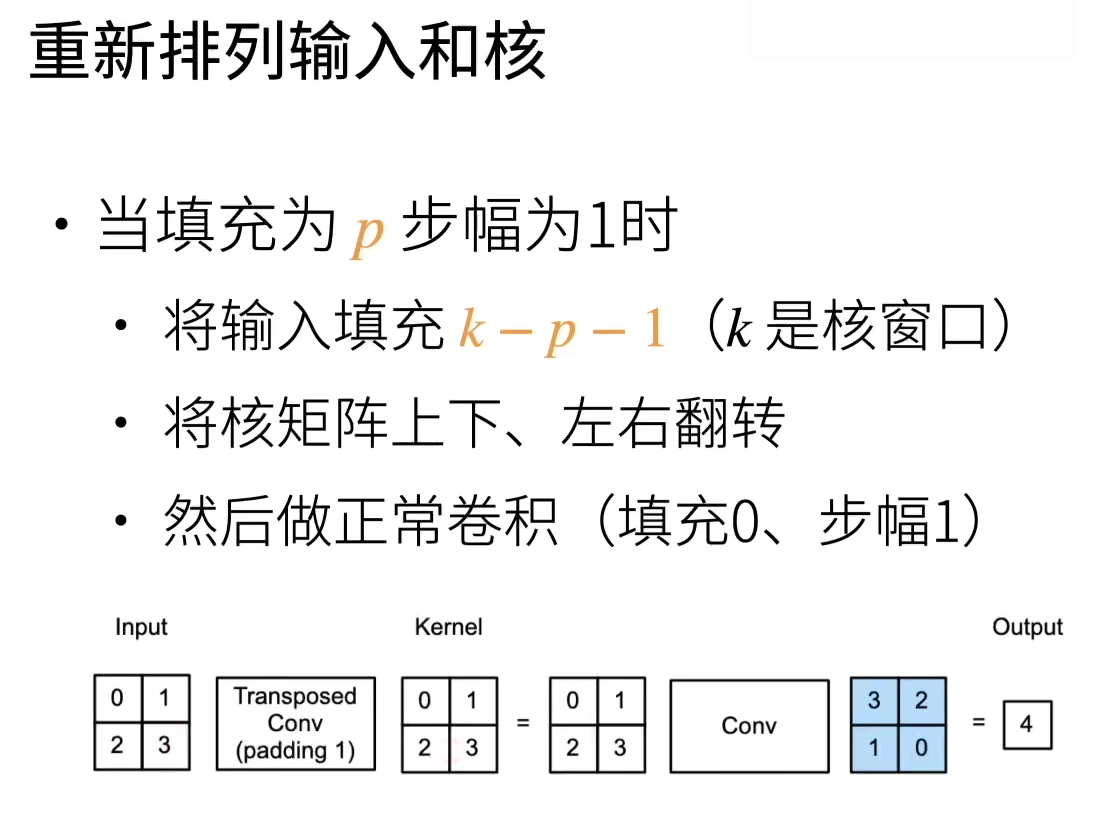
Set the padding=1 of the function, input the filling 2-1-1, turn the kernel matrix left and right, up and down, and convolute to transpose the convolution value.

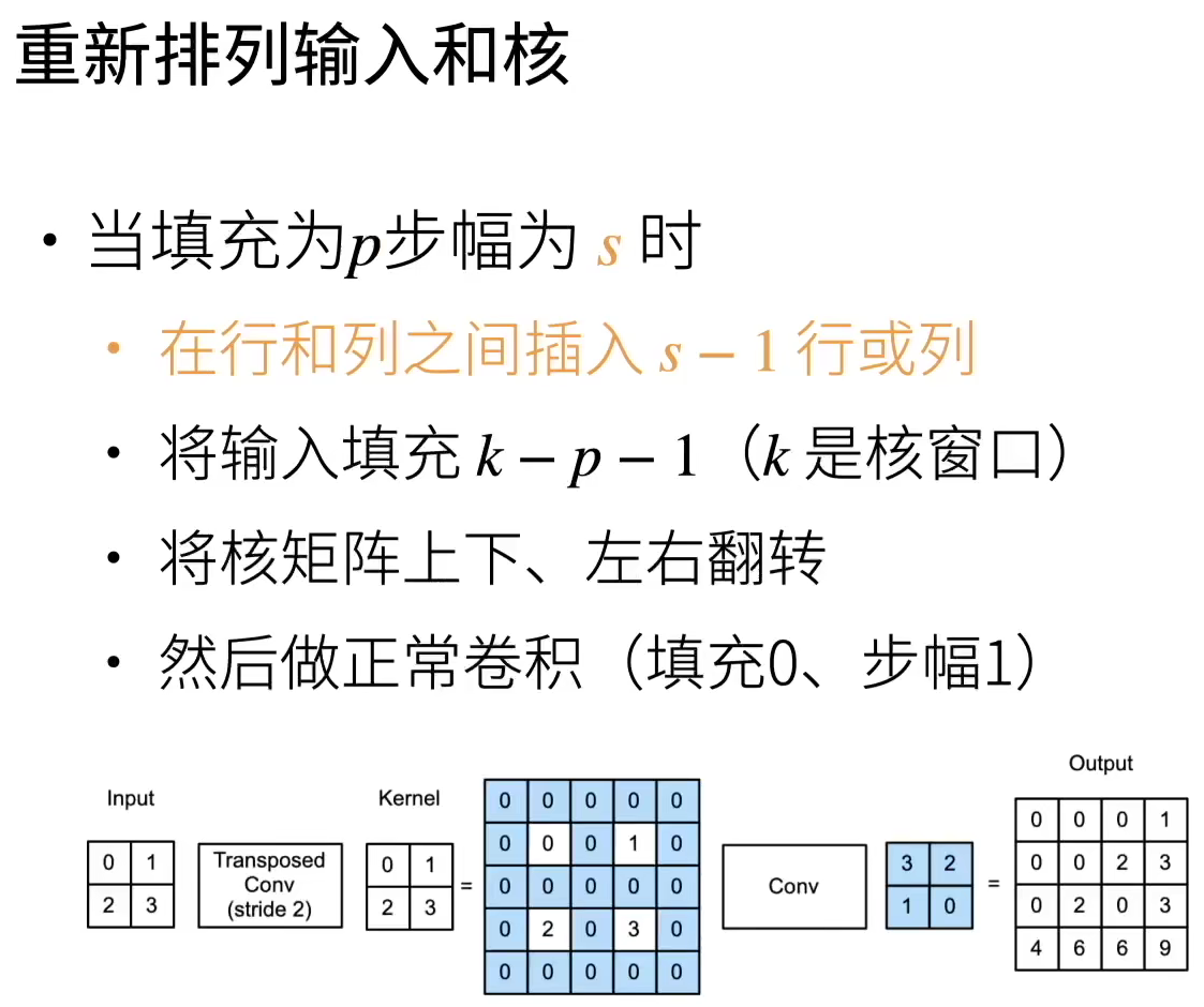
Set padding=1 for the function, and input padding 2-1-1; Set the function's stripe = 2 and insert 1 row or column between rows and columns. Turn the kernel matrix left and right, up and down, and convolute to transpose the convolution value.

10.5 relationship with deconvolution

10.6 summary

• Transposed convolution is contrary to the conventional convolution in which the input elements are reduced through the convolution kernel. Transposed convolution broadcasts the input elements through the convolution kernel, resulting in an output with a shape larger than the input.
• If we input x into the convolution layer f to obtain the output Y=f(X) and create a transposed convolution layer g with the same hyperparameter as f but the number of output channels is the number of channels in X, the shape of g(Y) will be the same as X.
• We can use matrix multiplication to realize convolution. Transposed convolution layer can exchange the forward propagation function and back propagation function of convolution layer.

11 fully connected convolutional neural network FCN

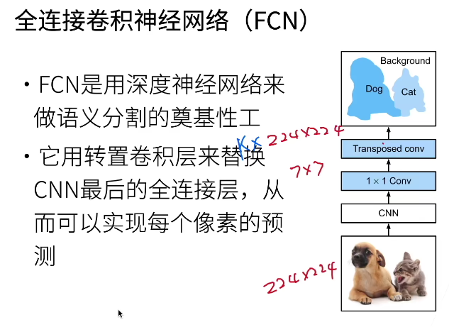
Semantic segmentation can classify each pixel in the image. Full convolutional network (FCN) uses convolutional neural network to realize the transformation from image pixels to pixel categories.

11.1 construction model

Full convolution network first uses convolution neural network to extract image features, and then through 1 × The convolution layer transforms the number of channels into the number of categories, and finally transforms the height and width of the feature image into the size of the input image through the transpose convolution layer. Therefore, the model output is the same as the height and width of the input image, and the final output channel includes the category prediction of the spatial position pixel.

We use ResNet-18 model pre trained on ImageNet dataset to extract image features, and record the network example as pre trained_ net. The last layers of the model include the global average aggregation layer and the fully connected layer, but they are not needed in the fully connected convolutional network.

pretrained_net = torchvision.models.resnet18(pretrained=True)
print(list(pretrained_net.children())[-3:])
###################
[Sequential(
   (0): BasicBlock(
     (conv1): Conv2d(256, 512, kernel_size=(3, 3), stride=(2, 2), padding=(1, 1), bias=False)
     (bn1): BatchNorm2d(512, eps=1e-05, momentum=0.1, affine=True, track_running_stats=True)
     (relu): ReLU(inplace=True)
     (conv2): Conv2d(512, 512, kernel_size=(3, 3), stride=(1, 1), padding=(1, 1), bias=False)
     (bn2): BatchNorm2d(512, eps=1e-05, momentum=0.1, affine=True, track_running_stats=True)
     (downsample): Sequential(
       (0): Conv2d(256, 512, kernel_size=(1, 1), stride=(2, 2), bias=False)
       (1): BatchNorm2d(512, eps=1e-05, momentum=0.1, affine=True, track_running_stats=True)
     )
   )
   (1): BasicBlock(
     (conv1): Conv2d(512, 512, kernel_size=(3, 3), stride=(1, 1), padding=(1, 1), bias=False)
     (bn1): BatchNorm2d(512, eps=1e-05, momentum=0.1, affine=True, track_running_stats=True)
     (relu): ReLU(inplace=True)
     (conv2): Conv2d(512, 512, kernel_size=(3, 3), stride=(1, 1), padding=(1, 1), bias=False)
     (bn2): BatchNorm2d(512, eps=1e-05, momentum=0.1, affine=True, track_running_stats=True)
   )
 ),
 # The last two floors don't!
 AdaptiveAvgPool2d(output_size=(1, 1)),
 Linear(in_features=512, out_features=1000, bias=True)]

Next, we create a full convolution network instance. net. It replicates most of the pre training layers in Resnet-18, but removes the final global average aggregation layer and the full connection layer closest to the output.

net = nn.Sequential(*list(pretrained_net.children())[:-2])

Given the input height and width of 320 and 480 respectively, the forward calculation of net reduces the input height and width to 1 / 32, that is, 10 and 15.

X = torch.rand(size=(1, 3, 320, 480))
print(net(X).shape)
# torch.Size([1, 512, 10, 15])

Next, we use 1 × 1. The convolution layer converts the number of output channels into the number of classes (21 classes) of Pascal VOC2012 data set.

num_classes = 21
net.add_module('final_conv', nn.Conv2d(512, num_classes, kernel_size=1))

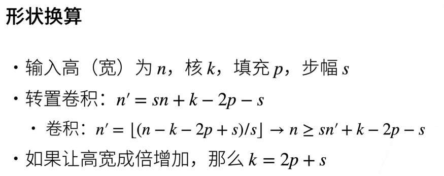
Finally, we need to increase the height and width of the feature map 32 times to change it back to the height and width of the input image. Recall the calculation method of the convolution output shape in section 6.3: due to (320 − 64 + 16 × 2 + 32) / 32 = 10 and (480 − 64 + 16) × 2 + 32) / 32 = 15, we construct a transposed convolution layer with a step of 32, and set the height and width of the convolution kernel to 64 and the filling to 16. We can see that if the step is s, the filling is s/2 (assuming that s/2 is an integer) and the height and width of the convolution kernel are 2s, the transposed convolution kernel will enlarge the input height and width by s times respectively.

net.add_module('transpose_conv', nn.ConvTranspose2d(num_classes, num_classes,
                                    kernel_size=64, padding=16, stride=32))

11.2 initialize transpose convolution

In image processing, it is sometimes necessary to enlarge the image, that is, upsampling. bilinear interpolation is one of the commonly used up sampling methods. It is also often used to initialize the transposed convolution layer.

To explain bilinear interpolation, assuming a given input image, we want to calculate each pixel on the upsampled output image. First, the coordinates (x,y) of the output image are mapped to the coordinates (x ', y') of the input image. For example, it is mapped according to the size ratio of input to output. Note that the mapped X 'and y' are real numbers. Then, four pixels closest to the coordinates (x ', y') are found on the input image. Finally, the pixels of the output image on the coordinates (x,y) are calculated according to the four pixels on the input image and their relative distance from (x ', y').

The up sampling of bilinear interpolation can be realized by transposing the convolution layer, and the kernel is composed of the following bilinear_kernel function construction.

def bilinear_kernel(in_channels, out_channels, kernel_size):
    factor = (kernel_size + 1) // 2
    if kernel_size % 2 == 1:
        center = factor - 1
    else:
        center = factor - 0.5
    og = (torch.arange(kernel_size).reshape(-1, 1),
          torch.arange(kernel_size).reshape(1, -1))
    filt = (1 - torch.abs(og[0] - center) / factor) * \
           (1 - torch.abs(og[1] - center) / factor)
    weight = torch.zeros((in_channels, out_channels,
                          kernel_size, kernel_size))
    weight[range(in_channels), range(out_channels), :, :] = filt
    return weight

Let's use the up sampling experiment of bilinear interpolation, which is realized by transposed convolution. We construct a transposed convolution layer that enlarges the input height and width twice, and use biliner as its convolution kernel_ Kernel function initialization.

conv_trans = nn.ConvTranspose2d(3, 3, kernel_size=4, padding=1, stride=2,
                                bias=False)
conv_trans.weight.data.copy_(bilinear_kernel(3, 3, 4));

Read the image X and record the result of up sampling as Y. In order to print the image, we need to adjust the position of the channel dimension.

img = torchvision.transforms.ToTensor()(d2l.Image.open('catdog.png'))
X = img.unsqueeze(0)
Y = conv_trans(X)
out_img = Y[0].permute(1, 2, 0).detach()

d2l.set_figsize()
print('input image shape:', img.permute(1, 2, 0).shape)
d2l.plt.imshow(img.permute(1, 2, 0));
print('output image shape:', out_img.shape)
d2l.plt.imshow(out_img)

img = torchvision.transforms.ToTensor()(d2l.Image.open('catdog.png'))
X = img.unsqueeze(0)
Y = conv_trans(X)
out_img = Y[0].permute(1, 2, 0).detach()

d2l.set_figsize()
print('input image shape:', img.permute(1, 2, 0).shape)
d2l.plt.imshow(img.permute(1, 2, 0));
print('output image shape:', out_img.shape)
d2l.plt.imshow(out_img)
plt.show()

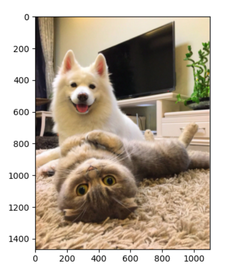
It can be seen that the transposed convolution layer enlarges the height and width of the image twice respectively. In addition to the different coordinate scales, the image enlarged by bilinear interpolation is the same as before.

11.3 reading data sets

Specifies that the shape of the randomly cropped output image is 320 × 480: both height and width can be divided by 32.

batch_size, crop_size = 32, (320, 480)
train_iter, test_iter = d2l.load_data_voc(batch_size, crop_size)
###############
read 1114 examples
read 1078 examples

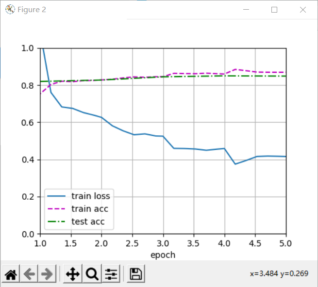
11.4 training

Now we can train the full convolution network. The loss function and accuracy calculation here are not essentially different from those in image classification, because we use the channel of transposed convolution layer to predict the category of pixels, so the channel dimension is specified in the loss calculation. In addition, the model calculates the accuracy based on whether the prediction category of each pixel is correct.

def loss(inputs, targets):
    return F.cross_entropy(inputs, targets, reduction='none').mean(1).mean(1)

num_epochs, lr, wd, devices = 5, 0.001, 1e-3, d2l.try_all_gpus()
trainer = torch.optim.SGD(net.parameters(), lr=lr, weight_decay=wd)
d2l.train_ch13(net, train_iter, test_iter, loss, trainer, num_epochs, devices)

plt.show()

11.5 forecast

In prediction, we need to standardize the input image in each channel and convert it into the four-dimensional input format required by convolutional neural network.

def predict(img):
    X = test_iter.dataset.normalize_image(img).unsqueeze(0)
    pred = net(X.to(devices[0])).argmax(dim=1)
    return pred.reshape(pred.shape[1], pred.shape[2])

To visualize the predicted categories for each pixel, we map the predicted categories back to their annotation colors in the dataset.

def label2image(pred):
    colormap = torch.tensor(d2l.VOC_COLORMAP, device=devices[0])
    X = pred.long()
    return colormap[X, :]

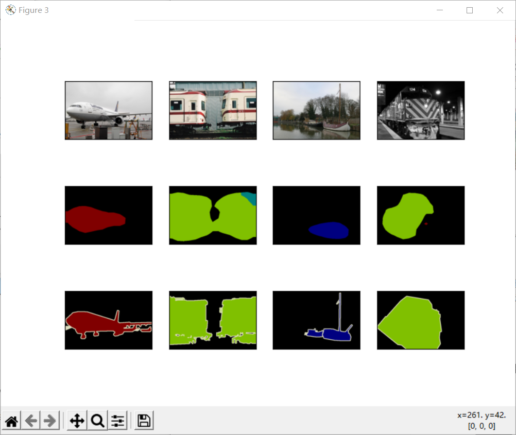
The images in the test dataset vary in size and shape. Because the model uses a transposed convolution layer with a step of 32, when the height or width of the input image cannot be divided by 32, the output height or width of the transposed convolution layer will deviate from the size of the input image. In order to solve this problem, multiple rectangular regions with an integer multiple of 32 in height and width can be intercepted in the image, and the pixels in these regions can be calculated forward respectively.

voc_dir = d2l.download_extract('voc2012', 'VOCdevkit/VOC2012')
test_images, test_labels = d2l.read_voc_images(voc_dir, False)
n, imgs = 4, []
for i in range(n):
    crop_rect = (0, 0, 320, 480)
    X = torchvision.transforms.functional.crop(test_images[i], *crop_rect)
    pred = label2image(predict(X))
    imgs += [X.permute(1,2,0), pred.cpu(),
             torchvision.transforms.functional.crop(
                 test_labels[i], *crop_rect).permute(1,2,0)]
d2l.show_images(imgs[::3] + imgs[1::3] + imgs[2::3], 3, n, scale=2);

11.6 summary

• Full convolution network first uses convolution neural network to extract image features, and then through 1 × The convolution layer transforms the number of channels into the number of categories, and finally transforms the height and width of the feature image into the size of the input image through the transpose convolution layer.
• In the full convolution network, we can initialize the transposed convolution layer as the up sampling of bilinear interpolation.

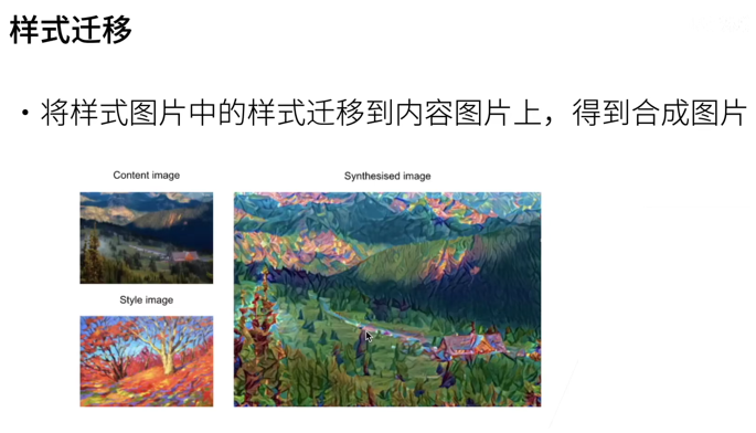
12 style migration

In this section, we will introduce how to use convolutional neural network to automatically apply the style in one image to another image, that is, style transfer.

12.1 method

A simple example is given to illustrate the style transfer method based on convolutional neural network.
① Initialize the composite image. The composite image is initialized to a content image,. The composite image is the only variable that needs to be updated in the style migration process, that is, the model parameters that need to be iterated in the style migration.
② A pre trained convolutional neural network is selected to extract the features of the image, and the model parameters do not need to be updated in the training. This deep convolution neural network extracts the image features level by level with multiple layers, and we can select the output of some of them as content features or style features.

As an example, the pre trained neural network selected here contains three convolution layers, in which the second layer outputs content features and the first and third layers output style features.

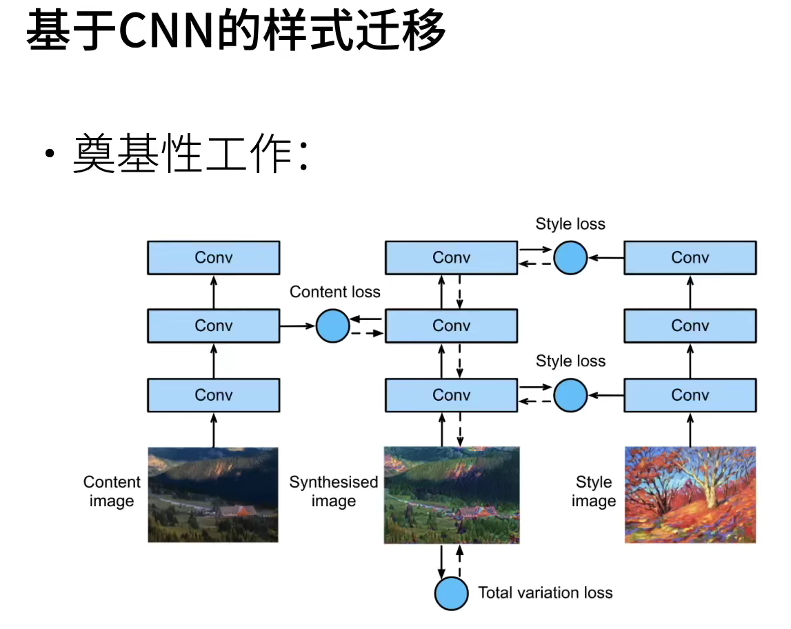
Next, we calculate the loss function of style migration through forward propagation (solid line arrow direction), and iterate the model parameters through back propagation (dotted line arrow direction), that is, constantly update the composite image.

The loss function commonly used in style migration consists of three parts:
(i) The content loss makes the composite image close to the content image in content features;
(ii) style loss makes the composite image close to the style image in style features;
(iii) the total variation loss helps to reduce the noise in the composite image.

Finally, when the model training is finished, we output the model parameters of style migration, that is, we get the final composite image.

12.2 reading content and style image

Read content and style images.

d2l.set_figsize()
content_img = d2l.Image.open('hills-ge2a578c6c_640.jpg')
style_img = d2l.Image.open('colorful-gd17f65ce2_640.jpg')

12.3 pretreatment and post-treatment

The preprocessing function preprocess standardizes the input image in the three RGB channels, and transforms the result into the input format accepted by the convolutional neural network.
The post-processing function postprocess restores the pixel values in the output image back to the values before standardization. Since the image printing function requires the floating-point value of each pixel to be between 0 and 1, we take 0 and 1 for values less than 0 and greater than 1 respectively.

rgb_mean = torch.tensor([0.485, 0.456, 0.406])
rgb_std = torch.tensor([0.229, 0.224, 0.225])

def preprocess(img, image_shape):
    transforms = torchvision.transforms.Compose([
        torchvision.transforms.Resize(image_shape),
        torchvision.transforms.ToTensor(),
        torchvision.transforms.Normalize(mean=rgb_mean, std=rgb_std)])
    return transforms(img).unsqueeze(0)

def postprocess(img):
    img = img[0].to(rgb_std.device)
    img = torch.clamp(img.permute(1, 2, 0) * rgb_std + rgb_mean, 0, 1)
    return torchvision.transforms.ToPILImage()(img.permute(2, 0, 1))

12.4 extracting image features

We use the VGG-19 model pre trained based on ImageNet dataset to extract image features [Gatys et al., 2016].

pretrained_net = torchvision.models.vgg19(pretrained=True)

In order to extract the content and style features of images, we can select the output of some layers in VGG network. Generally speaking, the closer to the input layer, the easier it is to extract the detail information of the image; On the contrary, the easier it is to extract the global information of the image.

In order to avoid too many composite images and preserve the details of the content image, we choose the layer closer to the output of VGG, that is, the content layer, to output the content features of the image. We also select the output of different layers from VGG to match the local and global styles. These layers are also called style layers.

The VGG network uses five convolution blocks. In the experiment, we select the last convolution layer of the fourth convolution block as the content layer and the first convolution layer of each convolution block as the style layer. The indexes of these layers can be pre trained by printing_ Net instance.

style_layers, content_layers = [0, 5, 10, 19, 28], [25]

When using VGG layer to extract features, we only need to use all layers from the input layer to the content layer or style layer closest to the output layer.

net = nn.Sequential(*[pretrained_net.features[i] for i in
                      range(max(content_layers + style_layers) + 1)])

Given the input X, if we simply call the forward calculation net(X), we can only get the output of the last layer. Since we also need the output of the middle layer, here we calculate layer by layer and retain the output of the content layer and the style layer.

def extract_features(X, content_layers, style_layers):
    contents = []
    styles = []
    for i in range(len(net)):
        X = net[i](X)
        if i in style_layers:
            styles.append(X)
        if i in content_layers:
            contents.append(X)
    return contents, styles

get_ The contents function extracts content features from the content image; get_ The styles function extracts style features from style images.
Because there is no need to change the model parameters of the pre trained VGG during training, we can extract the content features and style features before the beginning of training. Since the composite image is the iterative model parameter required for style migration, we can only call extract during the training process_ Features function to extract the content features and style features of the composite image.

def get_contents(image_shape, device):
    content_X = preprocess(content_img, image_shape).to(device)
    contents_Y, _ = extract_features(content_X, content_layers, style_layers)
    return content_X, contents_Y

def get_styles(image_shape, device):
    style_X = preprocess(style_img, image_shape).to(device)
    _, styles_Y = extract_features(style_X, content_layers, style_layers)
    return style_X, styles_Y

12.5 defining loss function

Loss function for style migration. It consists of three parts: content loss, style loss and total variation loss.

12.5.1 content loss

Similar to the loss function in linear regression, content loss measures the difference in content characteristics between synthetic image and content image by square error function.

def content_loss(Y_hat, Y):
    return torch.square(Y_hat - Y.detach()).mean()

12.5.2 style loss

Style loss is similar to content loss. It also measures the difference in style between synthetic image and style image by square error function.

def gram(X):
    num_channels, n = X.shape[1], X.numel() // X.shape[1]
    X = X.reshape((num_channels, n))
    return torch.matmul(X, X.T) / (num_channels * n)

def style_loss(Y_hat, gram_Y):
    return torch.square(gram(Y_hat) - gram_Y.detach()).mean()

12.5.3 total variation loss

Sometimes, we learn that there are a lot of high-frequency noise in the composite image, that is, there are particularly bright or dark particle pixels. A common noise reduction method is total variation noise reduction: suppose xi,j represents the pixel value at the coordinates (i,j), so as to reduce the total variation loss.

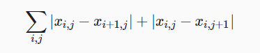
def tv_loss(Y_hat):
    return 0.5 * (torch.abs(Y_hat[:, :, 1:, :] - Y_hat[:, :, :-1, :]).mean() +
                  torch.abs(Y_hat[:, :, :, 1:] - Y_hat[:, :, :, :-1]).mean())

12.5.4 loss function

The loss function of style transfer is the weighted sum of content loss, style loss and total change loss. By adjusting these weight super parameters, we can weigh the relative importance of synthetic images in preserving content, migrating style and noise reduction.

content_weight, style_weight, tv_weight = 1, 1e3, 10

def compute_loss(X, contents_Y_hat, styles_Y_hat, contents_Y, styles_Y_gram):
    # Calculate the content loss, style loss and total variation loss respectively
    contents_l = [content_loss(Y_hat, Y) * content_weight for Y_hat, Y in zip(
        contents_Y_hat, contents_Y)]
    styles_l = [style_loss(Y_hat, Y) * style_weight for Y_hat, Y in zip(
        styles_Y_hat, styles_Y_gram)]
    tv_l = tv_loss(X) * tv_weight
    # Sum all losses
    l = sum(10 * styles_l + contents_l + [tv_l])
    return contents_l, styles_l, tv_l, l

12.6 initializing composite images

In style migration, the synthesized image is the only variable that needs to be updated during training. Therefore, we can define a simple model SynthesizedImage and treat the synthesized image as model parameters. The forward calculation of the model only needs to return the model parameters.

class SynthesizedImage(nn.Module):
    def __init__(self, img_shape, **kwargs):
        super(SynthesizedImage, self).__init__(**kwargs)
        self.weight = nn.Parameter(torch.rand(*img_shape))

    def forward(self):
        return self.weight

Next, we define get_inits function. This function creates a model instance of the composite image and initializes it to image X.

def get_inits(X, device, lr, styles_Y):
    gen_img = SynthesizedImage(X.shape).to(device)
    gen_img.weight.data.copy_(X.data)
    trainer = torch.optim.Adam(gen_img.parameters(), lr=lr)
    styles_Y_gram = [gram(Y) for Y in styles_Y]
    return gen_img(), styles_Y_gram, trainer

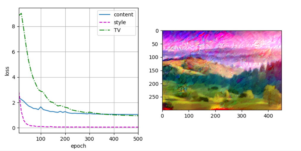
12.7 training model

In the training model for style transfer, we continuously extract the content features and style features of the synthetic image, and then calculate the loss function. The training cycle is defined below.

def train(X, contents_Y, styles_Y, device, lr, num_epochs, lr_decay_epoch):
    X, styles_Y_gram, trainer = get_inits(X, device, lr, styles_Y)
    scheduler = torch.optim.lr_scheduler.StepLR(trainer, lr_decay_epoch, 0.8)
    animator = d2l.Animator(xlabel='epoch', ylabel='loss',
                            xlim=[10, num_epochs],
                            legend=['content', 'style', 'TV'],
                            ncols=2, figsize=(7, 2.5))
    for epoch in range(num_epochs):
        trainer.zero_grad()
        contents_Y_hat, styles_Y_hat = extract_features(
            X, content_layers, style_layers)
        contents_l, styles_l, tv_l, l = compute_loss(
            X, contents_Y_hat, styles_Y_hat, contents_Y, styles_Y_gram)
        l.backward()
        trainer.step()
        scheduler.step()
        if (epoch + 1) % 10 == 0:
            animator.axes[1].imshow(postprocess(X))
            animator.add(epoch + 1, [float(sum(contents_l)),
                                     float(sum(styles_l)), float(tv_l)])
    return X

Now we train the model: first, adjust the height and width of the content image and the style image to 300 and 450 pixels respectively, and initialize the composite image with the content image.

device, image_shape = d2l.try_gpu(), (300, 450)
net = net.to(device)
content_X, contents_Y = get_contents(image_shape, device)
_, styles_Y = get_styles(image_shape, device)
output = train(content_X, contents_Y, styles_Y, device, 0.3, 500, 50)

12.8 summary

• The loss function commonly used in style migration consists of three parts: (i) content loss makes the composite image close to the content image in content features; (ii) the style loss makes the composite image close to the style image in style features; (iii) the total variation loss helps to reduce the noise in the composite image.
• We can extract the features of the image through the pre trained convolutional neural network, and continuously update the synthetic image as the model parameters by minimizing the loss function.