Reference book "deep learning practice" by Yang Yun and Du Fei
softmax implementation exercise
In the exercises in this chapter, we will gradually complete:
- 1. Be familiar with using CIFAR-10 dataset
- 2. Code softmax_ loss_ The naive function uses an explicit loop to calculate the loss function and the gradient
- 3. Code softmax_ loss_ The vectorized function uses the vectorized expression to calculate the loss function and the gradient
- 4. The coded minimum batch gradient descent algorithm trains the softmax classifier
- 5. Use validation data to select super parameters
#-*- coding: utf-8 -*-
import random
import numpy as np
from utils.data_utils import load_CIFAR10
from classifiers.chapter2 import *
import matplotlib.pyplot as plt

%matplotlib inline
plt.rcParams['figure.figsize'] = (10.0, 8.0)
%load_ext autoreload
%autoreload 2
# Import CIFAR-10 data
cifar10_dir = 'datasets\\cifar-10-batches-py'
X_train, y_train, X_test, y_test = load_CIFAR10(cifar10_dir)

# View data
print('Training data (number of data, data dimension): ', X_train.shape)
print('Training data markers (number of data markers,): ', y_train.shape)
print('Test data (number of data, data dimension): ', X_test.shape)
print('Test data markers (number of data markers,): ', y_test.shape)
Training data (number of data, data dimension):  (50000, 32, 32, 3)
Training data markers (number of data markers,):  (50000,)
Test data (number of data, data dimension):  (10000, 32, 32, 3)
Test data markers (number of data markers,):  (10000,)
# Data visualization
classes = ['plane', 'car', 'bird', 'cat', 'deer', 'dog', 'frog', 'horse', 'ship', 'truck']
# Total categories
num_classes = len(classes)
# Number of samples per category
samples_per_class = 7
for y, cls in enumerate(classes): # Loop the element position and element of the list, y represents the element position (0,num_class), cls element itself 'plane', etc
    # numpy.flatnonzero():
    # This function inputs a matrix and returns the position (index) of non-zero elements in the flattened matrix
    idxs = np.flatnonzero(y_train == y)  # Find the location of the y class in the label
    idxs = np.random.choice(idxs, samples_per_class, replace=False) #Select the seven samples we need
    for i, idx in enumerate(idxs): # Cycle the position of the selected sample and the position of the picture corresponding to the sample in the training set
        plt_idx = i * num_classes + y + 1  # Calculation of position in subgraph
        plt.subplot(samples_per_class, num_classes, plt_idx)  # Indicate the number of subgraphs to be drawn
        plt.imshow(X_train[idx].astype('uint8'))  # Drawing
        plt.axis('off')
        if i == 0:
            plt.title(cls)  # Write the title, that is, the class alias
plt.show()  # display

1. Data preprocessing
In general, we need to normalize the input data, that is, make the data have a standard normal distribution with zero mean and 1 variance. Since the feature range of the image is [0255], its variance has been constrained. We only need to centralize the data with zero mean, and there is no need to compress the data in the range of [- 1,1] (of course, you can also do this).
def get_CIFAR10_data(num_training=49000, num_validation=100, num_test=10000, num_sample=250):
    '''
    Skilled use CIFAR-10 data set
    CIFAR-10 The data set includes 60000 pieces with a size of 32*32 Ten categories of pictures.
    num_training: Number of training data samples
    num_validation: Number of validation data samples
    num_test: Number of test data samples
    num_sample: Sample data samples
    '''
    # Import CIFAR-10 data
    cifar10_dir = 'datasets/cifar-10-batches-py'
    X_train, y_train, X_test, y_test = load_CIFAR10(cifar10_dir)

    # Sampling data
    mask = range(num_training, num_training + num_validation)
    X_val = X_train[mask]
    y_val = y_train[mask]
    mask = range(num_training)
    X_train = X_train[mask]
    y_train = y_train[mask]
    mask = range(num_test)
    X_test = X_test[mask]
    y_test = y_test[mask]
    mask = np.random.choice(num_training, num_sample, replace=False)
    X_sample = X_train[mask]
    y_sample = y_train[mask]

    # Data shape conversion
    # Compress (width, height, color track) on one dimension
    # Reshape data into (number of data, dimension) shape
    X_train = np.reshape(X_train,(X_train.shape[0], -1))
    X_val = np.reshape(X_val,(X_val.shape[0], -1))
    X_test = np.reshape(X_test,(X_test.shape[0], -1))
    X_sample = np.reshape(X_sample,(X_sample.shape[0], -1))

    # data normalization
    # Data preprocessing, subtracting its mean
    mean_image = np.mean(X_train, axis = 0)
    X_train -= mean_image
    X_val -= mean_image
    X_test -= mean_image
    X_sample -= mean_image

    # Add an offset to each column of data
    # np.hstack superimposes the element array of parameter tuples horizontally
    X_train = np.hstack([X_train, np.ones((X_train.shape[0], 1))])
    X_val = np.hstack([X_val, np.ones((X_val.shape[0], 1))])
    X_test = np.hstack([X_test, np.ones((X_test.shape[0], 1))])
    X_sample = np.hstack([X_sample, np.ones((X_sample.shape[0], 1))])

    return X_train, y_train, X_val, y_val, X_test, y_test, X_sample, y_sample

X_train, y_train, X_val, y_val, X_test, y_test, X_sample, y_sample = get_CIFAR10_data()
print('Train data shape: ', X_train.shape)
print('Train labels shape: ', y_train.shape)
print('Validation data shape: ', X_val.shape)
print('Validation labels shape: ', y_val.shape)
print('Test data shape: ', X_test.shape)
print('Test labels shape: ', y_test.shape)
print('sample data shape: ', X_sample.shape)
print('sample labels shape: ', y_sample.shape)
Train data shape:  (49000, 3073)
Train labels shape:  (49000,)
Validation data shape:  (100, 3073)
Validation labels shape:  (100,)
Test data shape:  (10000, 3073)
Test labels shape:  (10000,)
sample data shape:  (250, 3073)
sample labels shape:  (250,)
2. Calculate the loss function and gradient using explicit loops
Please use as few loops as possible. The fewer loops you use, you can save more computing time. It is necessary to gradually adapt to vectorization calculation expression, because using vectorization expression can not only write a brief introduction, greatly improve the readability of the code, not easy to produce errors, but also greatly improve the operation efficiency.
# First, we will implement the loss function (cost function) of softmax in a circular way
# Open classifiers/chapter2/softmax_loss.py file and implement softmax_loss_naive function
# When finished, run the unit code
from classifiers.chapter2.softmax_loss import softmax_loss_naive
import time

# Initialize weight
W = np.random.randn(3073, 10) * 0.0001
loss, grad = softmax_loss_naive(W, X_sample, y_sample, 0.0)

# Your initialization loss value should be close to - log(0.1)
print('You achieved it softmax magnitude of the loss loss: %f' % loss)
print('Correct loss value: %f' % ( -np.log(0.1) ))
You achieved it softmax magnitude of the loss loss: 2.322683
 Correct loss value: 2.302585
# Use numerical gradients to test your implemented softmax_loss_naive
# The gradient you achieve should be close to the numerical gradient
from utils.gradient_check import grad_check_sparse
loss, grad = softmax_loss_naive(W, X_sample, y_sample, 0.0)

print('Check the weight attenuation softmax_loss_naive Gradient:')
f = lambda w: softmax_loss_naive(w, X_sample, y_sample, 0.0)[0]
grad_numerical = grad_check_sparse(f, W, grad, 10)

print('Check the weight after adding the weight attenuation term softmax_loss_naive Gradient:')
loss, grad = softmax_loss_naive(W, X_sample, y_sample, 1e2)
f = lambda w: softmax_loss_naive(w, X_sample, y_sample, 1e2)[0]
grad_numerical = grad_check_sparse(f, W, grad, 10)
Check the weight attenuation softmax_loss_naive Gradient:
numerical: -1.643731 analytic: -1.643731, relative error: 1.767333e-08
numerical: -0.903899 analytic: -0.903899, relative error: 4.933728e-08
numerical: -1.871885 analytic: -1.871886, relative error: 1.466657e-08
numerical: 1.315985 analytic: 1.315985, relative error: 2.012378e-08
numerical: 1.398138 analytic: 1.398138, relative error: 2.379984e-08
numerical: 0.787859 analytic: 0.787859, relative error: 3.121790e-08
numerical: -2.592382 analytic: -2.592382, relative error: 2.092500e-08
numerical: -2.854713 analytic: -2.854713, relative error: 7.280248e-09
numerical: 1.232664 analytic: 1.232664, relative error: 2.542693e-08
numerical: 1.706167 analytic: 1.706167, relative error: 3.109060e-08
 Check the weight after adding the weight attenuation term softmax_loss_naive Gradient:
numerical: -0.176439 analytic: -0.176439, relative error: 3.089932e-07
numerical: -3.940286 analytic: -3.940286, relative error: 7.815151e-09
numerical: -1.458173 analytic: -1.458173, relative error: 3.271034e-09
numerical: -0.478771 analytic: -0.478771, relative error: 9.152370e-09
numerical: -0.668009 analytic: -0.668009, relative error: 1.134638e-07
numerical: -1.660221 analytic: -1.660221, relative error: 1.547873e-08
numerical: 1.744188 analytic: 1.744188, relative error: 2.014491e-08
numerical: -0.485254 analytic: -0.485254, relative error: 5.129877e-08
numerical: -2.515499 analytic: -2.515499, relative error: 2.575850e-09
numerical: 2.403642 analytic: 2.403642, relative error: 1.413098e-08
3. Calculate the loss function and gradient using vectorization expression
# Now we will implement the vectorized softmax loss and its gradient calculation
# Open softmax_loss_vectorized function and complete the corresponding task, run the code
# The vectorized version should be the same as the explicit loop version, but the former should be much faster
tic = time.time()
loss_naive, grad_naive = softmax_loss_naive(W, X_sample, y_sample, 0.00001)
toc = time.time()
print('Explicit circular version loss: %e   Spend time %fs' % (loss_naive, toc - tic))

from classifiers.chapter2.softmax_loss import softmax_loss_vectorized
tic = time.time()
loss_vectorized, grad_vectorized = softmax_loss_vectorized(W, X_sample, y_sample, 0.00001)
toc = time.time()
print('Vectorized version loss: %e    Spend time %fs' % (loss_vectorized, toc - tic))

# Comparison results
grad_difference = np.linalg.norm(grad_naive - grad_vectorized, ord='fro')
print('Loss error: %f' % np.abs(loss_naive - loss_vectorized))
print('Gradient error: %f' % grad_difference)
Explicit circular version loss: 2.322683e+00   Time spent 0.101504s
 Vectorized version loss: 2.322683e+00    Time spent 0.001956s
 Loss error: 0.000000
 Gradient error: 0.000000
4. The minimum batch gradient descent algorithm trains the softmax classifier
# Open softmax.trian() to complete the random gradient descent task, and then execute the code
from classifiers.chapter2.softmax import *
softmax = Softmax()
tic = time.time()
loss_hist = softmax.train(X_sample, y_sample, learning_rate=1e-7, reg=5e4,
                      num_iters=3500, verbose=True)
toc = time.time()
print('Spend time %fs' % (toc - tic))
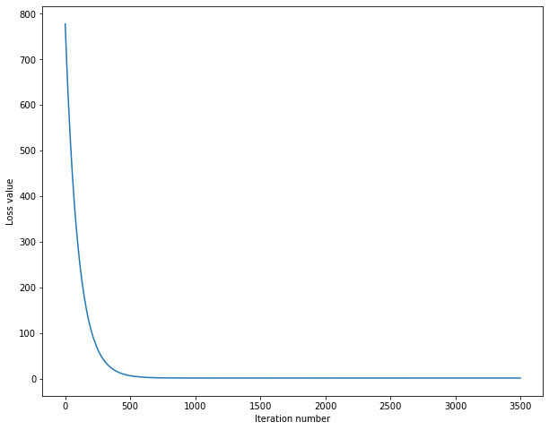
Iterations 0 / 3500: loss 777.592212
 Number of iterations 500 / 3500: loss 7.042712
 Number of iterations 1000 / 3500: loss 1.952050
 Number of iterations 1500 / 3500: loss 1.920996
 Number of iterations 2000 / 3500: loss 1.897792
 Number of iterations 2500 / 3500: loss 1.923868
 Number of iterations 3000 / 3500: loss 1.904769
 Take time 11.818226s
# View the change of loss value
plt.plot(loss_hist)
plt.xlabel('Iteration number')
plt.ylabel('Loss value')
plt.show()
# Test the training set and verify the accuracy of the set
y_train_pred = softmax.predict(X_sample)
print(y_train_pred.shape)
print('Amount of training data:%f    Training accuracy: %f' % (X_sample.shape[0],np.mean(y_sample == y_train_pred), ))
y_val_pred = softmax.predict(X_val)
print('Amount of validation data:%f    Verification accuracy: %f' % (X_val.shape[0],np.mean(y_val == y_val_pred), ))
(250,)
Training data volume: 250.000000    Training accuracy: 0.576000
 Amount of validation data: 100.000000    Verification accuracy: 0.240000
5. Use validation data to select super parameters
# Use the verification set to adjust the super parameters (weight, attenuation factor, learning rate)
from classifiers.chapter2.softmax import *
results = {}
best_val = -1
best_l = 0  # Best learning rate
best_r = 0  # Optimal weight attenuation factor
best_softmax = None
# Learning rate
learning_rates=np.logspace(-9, 0, num=10)
# Weight attenuation factor
regularization_strengths=np.logspace(0, 5, num=10)
batch_size = [50]
num_iters  = [300]

for b in batch_size:
    for n in num_iters:
        for l in learning_rates:
            for r in regularization_strengths:
                # Create a Softmax class for comparison
                softmax = Softmax()
                loss_hist = softmax.train(X_sample, y_sample,
                                         learning_rate=l,reg=r,
                                         num_iters=n,
                                         batch_size=b,
                                         verbose=False)
                y_train_pred = softmax.predict(X_sample)
                train_accuracy= np.mean(y_sample == y_train_pred)
                y_val_pred = softmax.predict(X_val)
                val_accuracy= np.mean(y_val == y_val_pred)
                results[(l,r)]=(train_accuracy,val_accuracy)
                # Find the parameter configuration with the highest accuracy
                if(best_val < val_accuracy):
                    best_val = val_accuracy
                    best_softmax = softmax
                    best_l =l
                    best_r =r

for lr, reg in sorted(results):
    train_accuracy, val_accuracy = results[(lr, reg)]
    print('lr %e reg %e Training accuracy: %f Verification accuracy: %f' % (
                lr, reg, train_accuracy, val_accuracy))

print('The best learning rate is:%e The best weight attenuation coefficient is:%e The corresponding verification accuracy is: %f' % (best_l,best_r,best_val))
lr 1.000000e-09 reg 1.000000e+00 Training accuracy: 0.152000 Verification accuracy: 0.120000
lr 1.000000e-09 reg 3.593814e+00 Training accuracy: 0.064000 Verification accuracy: 0.090000
lr 1.000000e-09 reg 1.291550e+01 Training accuracy: 0.116000 Verification accuracy: 0.170000
lr 1.000000e-09 reg 4.641589e+01 Training accuracy: 0.048000 Verification accuracy: 0.080000
lr 1.000000e-09 reg 1.668101e+02 Training accuracy: 0.104000 Verification accuracy: 0.150000
lr 1.000000e-09 reg 5.994843e+02 Training accuracy: 0.148000 Verification accuracy: 0.100000
lr 1.000000e-09 reg 2.154435e+03 Training accuracy: 0.096000 Verification accuracy: 0.090000
lr 1.000000e-09 reg 7.742637e+03 Training accuracy: 0.112000 Verification accuracy: 0.140000
lr 1.000000e-09 reg 2.782559e+04 Training accuracy: 0.064000 Verification accuracy: 0.100000
lr 1.000000e-09 reg 1.000000e+05 Training accuracy: 0.108000 Verification accuracy: 0.070000
lr 1.000000e-08 reg 1.000000e+00 Training accuracy: 0.108000 Verification accuracy: 0.060000
lr 1.000000e-08 reg 3.593814e+00 Training accuracy: 0.104000 Verification accuracy: 0.160000
lr 1.000000e-08 reg 1.291550e+01 Training accuracy: 0.092000 Verification accuracy: 0.110000
lr 1.000000e-08 reg 4.641589e+01 Training accuracy: 0.080000 Verification accuracy: 0.090000
lr 1.000000e-08 reg 1.668101e+02 Training accuracy: 0.136000 Verification accuracy: 0.090000
lr 1.000000e-08 reg 5.994843e+02 Training accuracy: 0.132000 Verification accuracy: 0.080000
lr 1.000000e-08 reg 2.154435e+03 Training accuracy: 0.080000 Verification accuracy: 0.080000
lr 1.000000e-08 reg 7.742637e+03 Training accuracy: 0.148000 Verification accuracy: 0.080000
lr 1.000000e-08 reg 2.782559e+04 Training accuracy: 0.104000 Verification accuracy: 0.080000
lr 1.000000e-08 reg 1.000000e+05 Training accuracy: 0.092000 Verification accuracy: 0.070000
lr 1.000000e-07 reg 1.000000e+00 Training accuracy: 0.216000 Verification accuracy: 0.170000
lr 1.000000e-07 reg 3.593814e+00 Training accuracy: 0.300000 Verification accuracy: 0.120000
lr 1.000000e-07 reg 1.291550e+01 Training accuracy: 0.276000 Verification accuracy: 0.150000
lr 1.000000e-07 reg 4.641589e+01 Training accuracy: 0.304000 Verification accuracy: 0.170000
lr 1.000000e-07 reg 1.668101e+02 Training accuracy: 0.252000 Verification accuracy: 0.180000
lr 1.000000e-07 reg 5.994843e+02 Training accuracy: 0.232000 Verification accuracy: 0.170000
lr 1.000000e-07 reg 2.154435e+03 Training accuracy: 0.224000 Verification accuracy: 0.140000
lr 1.000000e-07 reg 7.742637e+03 Training accuracy: 0.256000 Verification accuracy: 0.130000
lr 1.000000e-07 reg 2.782559e+04 Training accuracy: 0.376000 Verification accuracy: 0.240000
lr 1.000000e-07 reg 1.000000e+05 Training accuracy: 0.500000 Verification accuracy: 0.210000
lr 1.000000e-06 reg 1.000000e+00 Training accuracy: 0.856000 Verification accuracy: 0.190000
lr 1.000000e-06 reg 3.593814e+00 Training accuracy: 0.872000 Verification accuracy: 0.200000
lr 1.000000e-06 reg 1.291550e+01 Training accuracy: 0.864000 Verification accuracy: 0.170000
lr 1.000000e-06 reg 4.641589e+01 Training accuracy: 0.852000 Verification accuracy: 0.200000
lr 1.000000e-06 reg 1.668101e+02 Training accuracy: 0.828000 Verification accuracy: 0.190000
lr 1.000000e-06 reg 5.994843e+02 Training accuracy: 0.868000 Verification accuracy: 0.240000
lr 1.000000e-06 reg 2.154435e+03 Training accuracy: 0.876000 Verification accuracy: 0.220000
lr 1.000000e-06 reg 7.742637e+03 Training accuracy: 0.808000 Verification accuracy: 0.240000
lr 1.000000e-06 reg 2.782559e+04 Training accuracy: 0.600000 Verification accuracy: 0.200000
lr 1.000000e-06 reg 1.000000e+05 Training accuracy: 0.404000 Verification accuracy: 0.190000
lr 1.000000e-05 reg 1.000000e+00 Training accuracy: 1.000000 Verification accuracy: 0.230000
lr 1.000000e-05 reg 3.593814e+00 Training accuracy: 1.000000 Verification accuracy: 0.170000
lr 1.000000e-05 reg 1.291550e+01 Training accuracy: 1.000000 Verification accuracy: 0.230000
lr 1.000000e-05 reg 4.641589e+01 Training accuracy: 1.000000 Verification accuracy: 0.210000
lr 1.000000e-05 reg 1.668101e+02 Training accuracy: 1.000000 Verification accuracy: 0.200000
lr 1.000000e-05 reg 5.994843e+02 Training accuracy: 0.996000 Verification accuracy: 0.210000
lr 1.000000e-05 reg 2.154435e+03 Training accuracy: 0.644000 Verification accuracy: 0.200000
lr 1.000000e-05 reg 7.742637e+03 Training accuracy: 0.460000 Verification accuracy: 0.210000
lr 1.000000e-05 reg 2.782559e+04 Training accuracy: 0.224000 Verification accuracy: 0.260000
lr 1.000000e-05 reg 1.000000e+05 Training accuracy: 0.140000 Verification accuracy: 0.080000
lr 1.000000e-04 reg 1.000000e+00 Training accuracy: 1.000000 Verification accuracy: 0.160000
lr 1.000000e-04 reg 3.593814e+00 Training accuracy: 1.000000 Verification accuracy: 0.160000
lr 1.000000e-04 reg 1.291550e+01 Training accuracy: 1.000000 Verification accuracy: 0.220000
lr 1.000000e-04 reg 4.641589e+01 Training accuracy: 1.000000 Verification accuracy: 0.210000
lr 1.000000e-04 reg 1.668101e+02 Training accuracy: 0.564000 Verification accuracy: 0.180000
lr 1.000000e-04 reg 5.994843e+02 Training accuracy: 0.492000 Verification accuracy: 0.190000
lr 1.000000e-04 reg 2.154435e+03 Training accuracy: 0.160000 Verification accuracy: 0.150000
lr 1.000000e-04 reg 7.742637e+03 Training accuracy: 0.160000 Verification accuracy: 0.120000
lr 1.000000e-04 reg 2.782559e+04 Training accuracy: 0.052000 Verification accuracy: 0.050000
lr 1.000000e-04 reg 1.000000e+05 Training accuracy: 0.092000 Verification accuracy: 0.110000
lr 1.000000e-03 reg 1.000000e+00 Training accuracy: 1.000000 Verification accuracy: 0.190000
lr 1.000000e-03 reg 3.593814e+00 Training accuracy: 1.000000 Verification accuracy: 0.180000
lr 1.000000e-03 reg 1.291550e+01 Training accuracy: 0.700000 Verification accuracy: 0.200000
lr 1.000000e-03 reg 4.641589e+01 Training accuracy: 0.304000 Verification accuracy: 0.160000
lr 1.000000e-03 reg 1.668101e+02 Training accuracy: 0.216000 Verification accuracy: 0.180000
lr 1.000000e-03 reg 5.994843e+02 Training accuracy: 0.116000 Verification accuracy: 0.130000
lr 1.000000e-03 reg 2.154435e+03 Training accuracy: 0.084000 Verification accuracy: 0.210000
lr 1.000000e-03 reg 7.742637e+03 Training accuracy: 0.104000 Verification accuracy: 0.100000
lr 1.000000e-03 reg 2.782559e+04 Training accuracy: 0.112000 Verification accuracy: 0.070000
lr 1.000000e-03 reg 1.000000e+05 Training accuracy: 0.112000 Verification accuracy: 0.070000
lr 1.000000e-02 reg 1.000000e+00 Training accuracy: 0.692000 Verification accuracy: 0.190000
lr 1.000000e-02 reg 3.593814e+00 Training accuracy: 0.380000 Verification accuracy: 0.180000
lr 1.000000e-02 reg 1.291550e+01 Training accuracy: 0.340000 Verification accuracy: 0.160000
lr 1.000000e-02 reg 4.641589e+01 Training accuracy: 0.148000 Verification accuracy: 0.090000
lr 1.000000e-02 reg 1.668101e+02 Training accuracy: 0.112000 Verification accuracy: 0.060000
lr 1.000000e-02 reg 5.994843e+02 Training accuracy: 0.076000 Verification accuracy: 0.060000
lr 1.000000e-02 reg 2.154435e+03 Training accuracy: 0.112000 Verification accuracy: 0.070000
lr 1.000000e-02 reg 7.742637e+03 Training accuracy: 0.112000 Verification accuracy: 0.070000
lr 1.000000e-02 reg 2.782559e+04 Training accuracy: 0.112000 Verification accuracy: 0.070000
lr 1.000000e-02 reg 1.000000e+05 Training accuracy: 0.112000 Verification accuracy: 0.070000
lr 1.000000e-01 reg 1.000000e+00 Training accuracy: 0.292000 Verification accuracy: 0.200000
lr 1.000000e-01 reg 3.593814e+00 Training accuracy: 0.196000 Verification accuracy: 0.180000
lr 1.000000e-01 reg 1.291550e+01 Training accuracy: 0.124000 Verification accuracy: 0.110000
lr 1.000000e-01 reg 4.641589e+01 Training accuracy: 0.116000 Verification accuracy: 0.170000
lr 1.000000e-01 reg 1.668101e+02 Training accuracy: 0.112000 Verification accuracy: 0.070000
lr 1.000000e-01 reg 5.994843e+02 Training accuracy: 0.112000 Verification accuracy: 0.070000
lr 1.000000e-01 reg 2.154435e+03 Training accuracy: 0.112000 Verification accuracy: 0.070000
lr 1.000000e-01 reg 7.742637e+03 Training accuracy: 0.112000 Verification accuracy: 0.070000
lr 1.000000e-01 reg 2.782559e+04 Training accuracy: 0.112000 Verification accuracy: 0.070000
lr 1.000000e-01 reg 1.000000e+05 Training accuracy: 0.112000 Verification accuracy: 0.070000
lr 1.000000e+00 reg 1.000000e+00 Training accuracy: 0.108000 Verification accuracy: 0.200000
lr 1.000000e+00 reg 3.593814e+00 Training accuracy: 0.108000 Verification accuracy: 0.050000
lr 1.000000e+00 reg 1.291550e+01 Training accuracy: 0.112000 Verification accuracy: 0.070000
lr 1.000000e+00 reg 4.641589e+01 Training accuracy: 0.112000 Verification accuracy: 0.070000
lr 1.000000e+00 reg 1.668101e+02 Training accuracy: 0.112000 Verification accuracy: 0.070000
lr 1.000000e+00 reg 5.994843e+02 Training accuracy: 0.112000 Verification accuracy: 0.070000
lr 1.000000e+00 reg 2.154435e+03 Training accuracy: 0.112000 Verification accuracy: 0.070000
lr 1.000000e+00 reg 7.742637e+03 Training accuracy: 0.112000 Verification accuracy: 0.070000
lr 1.000000e+00 reg 2.782559e+04 Training accuracy: 0.112000 Verification accuracy: 0.070000
lr 1.000000e+00 reg 1.000000e+05 Training accuracy: 0.112000 Verification accuracy: 0.070000
 The best learning rate is: 1.000000e-05 The best weight attenuation coefficient is: 2.782559e+04 The corresponding verification accuracy is: 0.260000
import math
# Generate corresponding point graph
x_scatter = [math.log10(x[0]) for x in results]
y_scatter = [math.log10(x[1]) for x in results]

# Accuracy of drawing training data
marker_size = 100
# Production color
colors = [results[x][0] for x in results]
plt.subplot(2, 1, 1)
# Draw corresponding points
plt.scatter(x_scatter, y_scatter, marker_size, c=colors)
# Add color column
plt.colorbar()
plt.xlabel('log learning rate')
plt.ylabel('log regularization strength')
plt.title('CIFAR-10 training accuracy')

# Drawing verification data accuracy
colors = [results[x][1] for x in results]
plt.subplot(2, 1, 2)
# Draw corresponding points
plt.scatter(x_scatter, y_scatter, marker_size, c=colors)
# Add color column
plt.colorbar()
plt.xlabel('log learning rate')
plt.ylabel('log regularization strength')
plt.title('CIFAR-10 validation accuracy')
# Automatic layout
plt.tight_layout()
plt.show()
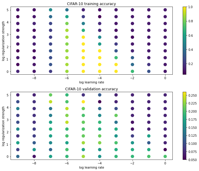
It can be clearly seen from the visualization results that the learning rate is about [1e-6, 1e-4], the effect is significant, and the penalty factor is better between [1e0, 1e4], and the smaller the penalty factor is, the better the effect may be. Therefore, our next step is to continue to narrow the scope.
#Use the verification set to adjust the super parameters (weight, attenuation factor, learning rate)
from classifiers.chapter2.softmax import *
results = {}
best_val = -1
best_l = 0
best_r = 0
best_softmax = None
learning_rates=np.logspace(-6, -4, num=10)
regularization_strengths=np.logspace(-1, 4, num=5)
batch_size = [50]
num_iters  = [300]

for b in batch_size:
    for n in num_iters:
        for l in learning_rates:
            for r in regularization_strengths:
                softmax = Softmax()
                loss_hist = softmax.train(X_sample, y_sample,
                                         learning_rate=l, reg=r,
                                         num_iters=n,batch_size=b, verbose=False)
                y_train_pred = softmax.predict(X_sample)
                train_accuracy= np.mean(y_sample == y_train_pred)
                y_val_pred = softmax.predict(X_val)
                val_accuracy= np.mean(y_val == y_val_pred)
                results[(l,r)]=(train_accuracy,val_accuracy)
                if (best_val < val_accuracy):
                    best_val = val_accuracy
                    best_softmax = softmax
                    best_l =l
                    best_r =r


print('The best learning rate is:%e The best weight attenuation coefficient is:%e The corresponding verification accuracy is: %f' % (best_l,best_r,best_val))
D:\workspace\Python\jupyter\Practical examples of in-depth learning\DLAction\classifiers\chapter2\softmax_loss.py:111: RuntimeWarning: divide by zero encountered in log
  loss += -np.sum(y_trueClass*np.log(prob))/num_train+0.5*reg*np.sum(W*W)
D:\workspace\Python\jupyter\Practical examples of in-depth learning\DLAction\classifiers\chapter2\softmax_loss.py:111: RuntimeWarning: invalid value encountered in multiply
  loss += -np.sum(y_trueClass*np.log(prob))/num_train+0.5*reg*np.sum(W*W)


The best learning rate is: 1.291550e-05 The best weight attenuation coefficient is: 1.000000e+04 The corresponding verification accuracy is: 0.240000
import math
x_scatter = [math.log10(x[0]) for x in results]
y_scatter = [math.log10(x[1]) for x in results]


# Accuracy of drawing training data
marker_size = 100
colors = [results[x][0] for x in results]
plt.subplot(2, 1, 1)
plt.scatter(x_scatter, y_scatter, marker_size, c=colors)
plt.colorbar()
plt.xlabel('log learning rate')
plt.ylabel('log regularization strength')
plt.title('CIFAR-10 training accuracy')

#Drawing verification data accuracy
colors = [results[x][1] for x in results]
plt.subplot(2, 1, 2)
plt.scatter(x_scatter, y_scatter, marker_size, c=colors)
plt.colorbar()
plt.xlabel('log learning rate')
plt.ylabel('log regularization strength')
plt.title('CIFAR-10 validation accuracy')
# Automatic layout
plt.tight_layout()
plt.show()
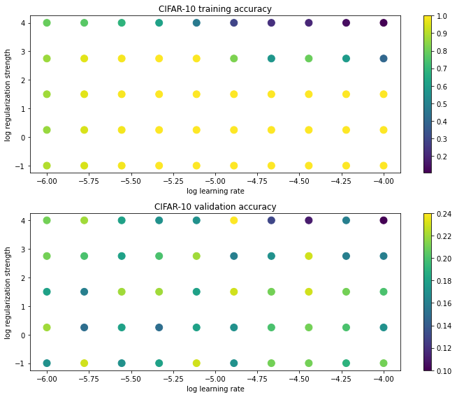
Continue to narrow the parameter range.
#Use the verification set to adjust the super parameters (weight, attenuation factor, learning rate)
from classifiers.chapter2.softmax import *
results = {}
best_val = -1
best_l = 0
best_r = 0
best_softmax = None
learning_rates=np.logspace(-5, -4, num=10)
regularization_strengths=np.logspace(-2, 3, num=5)
batch_size = [50]
num_iters  = [300]

for b in batch_size:
    for n in num_iters:
        for l in learning_rates:
            for r in regularization_strengths:
                softmax = Softmax()
                loss_hist = softmax.train(X_sample, y_sample, learning_rate=l,
                                         reg=r,num_iters=n,batch_size=b, verbose=False)
                y_train_pred = softmax.predict(X_sample)
                train_accuracy= np.mean(y_sample == y_train_pred)
                y_val_pred = softmax.predict(X_val)
                val_accuracy= np.mean(y_val == y_val_pred)
                results[(l,r)]=(train_accuracy,val_accuracy)
                if (best_val < val_accuracy):
                    best_val = val_accuracy
                    best_softmax = softmax
                    best_l =l
                    best_r =r

print('The best learning rate is:%e The best weight attenuation coefficient is:%e The corresponding verification accuracy is: %f' % (best_l,best_r,best_val))
The best learning rate is: 1.000000e-05 The best weight attenuation coefficient is: 3.162278e+00 The corresponding verification accuracy is: 0.230000
import math
x_scatter = [math.log10(x[0]) for x in results]
y_scatter = [math.log10(x[1]) for x in results]

marker_size = 100
colors = [results[x][0] for x in results]
plt.subplot(2, 1, 1)
plt.scatter(x_scatter, y_scatter, marker_size, c=colors)
plt.colorbar()
plt.xlabel('log learning rate')
plt.ylabel('log regularization strength')
plt.title('CIFAR-10 training accuracy')


colors = [results[x][1] for x in results]
plt.subplot(2, 1, 2)
plt.scatter(x_scatter, y_scatter, marker_size, c=colors)
plt.colorbar()
plt.xlabel('log learning rate')
plt.ylabel('log regularization strength')
plt.title('CIFAR-10 validation accuracy')
# Automatic layout
plt.tight_layout()
plt.show()

#Evaluate the best softmax classifier on the test data set
y_test_pred = best_softmax.predict(X_test)
test_accuracy = np.mean(y_test == y_test_pred)
print('Test set accuracy: %f' % test_accuracy)
Test set accuracy: 0.234500
We observed that the effect was not ideal because the amount of data we trained was too small.
Increasing the amount of data can avoid the occurrence of over fitting, but it also makes us time-consuming and labor-consuming in selecting super parameters. Therefore, we can use smaller data to roughly select the value range of super parameters, which can save training time. However, the superparameter that performs best in small data does not necessarily perform better when the amount of data is large. Therefore, we need to pay attention to the control of the amount of data, but this is a very empirical problem, which needs to accumulate admiration from a large number of experiments and keep trying. Remember, don't be afraid of mistakes.
def get_CIFAR10_data(num_training=49000, num_validation=1000, num_test=10000):
    cifar10_dir = 'datasets/cifar-10-batches-py'
    X_train, y_train, X_test, y_test = load_CIFAR10(cifar10_dir)
    mask = range(num_training, num_training + num_validation)
    X_val = X_train[mask]
    y_val = y_train[mask]
    mask = range(num_training)
    X_train = X_train[mask]
    y_train = y_train[mask]
    mask = range(num_test)
    X_test = X_test[mask]
    y_test = y_test[mask]
    X_train = np.reshape(X_train, (X_train.shape[0], -1))
    X_val = np.reshape(X_val, (X_val.shape[0], -1))
    X_test = np.reshape(X_test, (X_test.shape[0], -1))
    mean_image = np.mean(X_train, axis = 0)
    X_train -= mean_image
    X_val -= mean_image
    X_test -= mean_image
    X_train = np.hstack([X_train, np.ones((X_train.shape[0], 1))])
    X_val = np.hstack([X_val, np.ones((X_val.shape[0], 1))])
    X_test = np.hstack([X_test, np.ones((X_test.shape[0], 1))])
    return X_train, y_train, X_val, y_val, X_test, y_test


X_train, y_train, X_val, y_val, X_test, y_test = get_CIFAR10_data()
print ('Train data shape: ', X_train.shape)
print ('Train labels shape: ', y_train.shape)
print ('Validation data shape: ', X_val.shape)
print ('Validation labels shape: ', y_val.shape)
print ('Test data shape: ', X_test.shape)
print ('Test labels shape: ', y_test.shape)
Train data shape:  (49000, 3073)
Train labels shape:  (49000,)
Validation data shape:  (1000, 3073)
Validation labels shape:  (1000,)
Test data shape:  (10000, 3073)
Test labels shape:  (10000,)
from classifiers.chapter2.softmax  import Softmax
results = {}
best_val = -1
best_softmax = None
################################################################################
#                            task:                                             #
#               Use all training data to train a best softmax                            #
################################################################################
learning_rates = [1.4e-7, 1.45e-7, 1.5e-7, 1.55e-7, 1.6e-7]  #Learning rate
regularization_strengths = [2.3e4, 2.6e4, 2.7e4, 2.8e4, 2.9e4]  #Weight attenuation factor
for l in learning_rates:
    for r in regularization_strengths:
        softmax = Softmax()
        loss_hist = softmax.train(X_train, y_train, learning_rate=l,
                                  reg=r,num_iters=2000, verbose=True)
        y_train_pred = softmax.predict(X_train)
        train_accuracy= np.mean(y_train == y_train_pred)
        y_val_pred = softmax.predict(X_val)
        val_accuracy= np.mean(y_val == y_val_pred)
        results[(l,r)]=(train_accuracy,val_accuracy)
        if (best_val < val_accuracy):
            best_val = val_accuracy
            best_softmax = softmax
################################################################################
#                            End coding                                          #
################################################################################

for lr, reg in sorted(results):
    train_accuracy, val_accuracy = results[(lr, reg)]
    print('lr %e reg %e train accuracy: %f val accuracy: %f' % (
                lr, reg, train_accuracy, val_accuracy))

print('The best verification accuracy is: %f' % best_val)
Iterations 0 / 2000: loss 362.275538
 Number of iterations 500 / 2000: loss 15.973378
 Number of iterations 1000 / 2000: loss 2.563832
 Number of iterations 1500 / 2000: loss 2.039525
 Iterations 0 / 2000: loss 402.579894
 Number of iterations 500 / 2000: loss 12.217043
 Number of iterations 1000 / 2000: loss 2.312635
 Number of iterations 1500 / 2000: loss 2.033261
 Iterations 0 / 2000: loss 420.798641
 Number of iterations 500 / 2000: loss 11.346001
 Number of iterations 1000 / 2000: loss 2.314607
 Number of iterations 1500 / 2000: loss 2.044269
 Iterations 0 / 2000: loss 440.503492
 Number of iterations 500 / 2000: loss 10.521333
 Number of iterations 1000 / 2000: loss 2.191913
 Number of iterations 1500 / 2000: loss 2.124927
 Iterations 0 / 2000: loss 453.308193
 Number of iterations 500 / 2000: loss 9.689195
 Number of iterations 1000 / 2000: loss 2.130514
 Number of iterations 1500 / 2000: loss 2.027209
 Iterations 0 / 2000: loss 362.176210
 Number of iterations 500 / 2000: loss 14.451922
 Number of iterations 1000 / 2000: loss 2.447913
 Number of iterations 1500 / 2000: loss 2.041807
 Iterations 0 / 2000: loss 402.706053
 Number of iterations 500 / 2000: loss 11.013674
 Number of iterations 1000 / 2000: loss 2.216208
 Number of iterations 1500 / 2000: loss 2.032448
 Iterations 0 / 2000: loss 421.450555
 Number of iterations 500 / 2000: loss 10.149416
 Number of iterations 1000 / 2000: loss 2.186461
 Number of iterations 1500 / 2000: loss 2.062753
 Iterations 0 / 2000: loss 431.157711
 Number of iterations 500 / 2000: loss 9.254785
 Number of iterations 1000 / 2000: loss 2.161939
 Number of iterations 1500 / 2000: loss 1.991775
 Iterations 0 / 2000: loss 444.492450
 Number of iterations 500 / 2000: loss 8.409564
 Number of iterations 1000 / 2000: loss 2.136935
 Number of iterations 1500 / 2000: loss 1.971083
 Iterations 0 / 2000: loss 362.221476
 Number of iterations 500 / 2000: loss 13.076090
 Number of iterations 1000 / 2000: loss 2.398948
 Number of iterations 1500 / 2000: loss 1.981336
 Iterations 0 / 2000: loss 404.341723
 Number of iterations 500 / 2000: loss 9.917005
 Number of iterations 1000 / 2000: loss 2.178486
 Number of iterations 1500 / 2000: loss 1.977197
 Iterations 0 / 2000: loss 422.058121
 Number of iterations 500 / 2000: loss 9.169317
 Number of iterations 1000 / 2000: loss 2.147070
 Number of iterations 1500 / 2000: loss 2.085903
 Iterations 0 / 2000: loss 430.965383
 Number of iterations 500 / 2000: loss 8.230988
 Number of iterations 1000 / 2000: loss 2.127792
 Number of iterations 1500 / 2000: loss 1.982288
 Iterations 0 / 2000: loss 449.796595
 Number of iterations 500 / 2000: loss 7.626812
 Number of iterations 1000 / 2000: loss 2.066997
 Number of iterations 1500 / 2000: loss 2.038826
 Iterations 0 / 2000: loss 355.354397
 Number of iterations 500 / 2000: loss 11.726022
 Number of iterations 1000 / 2000: loss 2.327054
 Number of iterations 1500 / 2000: loss 1.960372
 Iterations 0 / 2000: loss 408.173326
 Number of iterations 500 / 2000: loss 8.995592
 Number of iterations 1000 / 2000: loss 2.188157
 Number of iterations 1500 / 2000: loss 2.035182
 Iterations 0 / 2000: loss 416.190544
 Number of iterations 500 / 2000: loss 8.098396
 Number of iterations 1000 / 2000: loss 2.138810
 Number of iterations 1500 / 2000: loss 2.016468
 Iterations 0 / 2000: loss 435.709668
 Number of iterations 500 / 2000: loss 7.583673
 Number of iterations 1000 / 2000: loss 2.123043
 Number of iterations 1500 / 2000: loss 2.050762
 Iterations 0 / 2000: loss 455.764297
 Number of iterations 500 / 2000: loss 6.993459
 Number of iterations 1000 / 2000: loss 2.058059
 Number of iterations 1500 / 2000: loss 1.998903
 Iterations 0 / 2000: loss 360.201729
 Number of iterations 500 / 2000: loss 10.908834
 Number of iterations 1000 / 2000: loss 2.237939
 Number of iterations 1500 / 2000: loss 2.049242
 Iterations 0 / 2000: loss 406.568389
 Number of iterations 500 / 2000: loss 8.150559
 Number of iterations 1000 / 2000: loss 2.124073
 Number of iterations 1500 / 2000: loss 2.041791
 Iterations 0 / 2000: loss 418.556158
 Number of iterations 500 / 2000: loss 7.397969
 Number of iterations 1000 / 2000: loss 2.090971
 Number of iterations 1500 / 2000: loss 2.099561
 Iterations 0 / 2000: loss 434.558226
 Number of iterations 500 / 2000: loss 6.857017
 Number of iterations 1000 / 2000: loss 2.133622
 Number of iterations 1500 / 2000: loss 2.058132
 Iterations 0 / 2000: loss 444.248523
 Number of iterations 500 / 2000: loss 6.207619
 Number of iterations 1000 / 2000: loss 2.031800
 Number of iterations 1500 / 2000: loss 1.994766
lr 1.400000e-07 reg 2.300000e+04 train accuracy: 0.351163 val accuracy: 0.367000
lr 1.400000e-07 reg 2.600000e+04 train accuracy: 0.349898 val accuracy: 0.365000
lr 1.400000e-07 reg 2.700000e+04 train accuracy: 0.347102 val accuracy: 0.360000
lr 1.400000e-07 reg 2.800000e+04 train accuracy: 0.344673 val accuracy: 0.359000
lr 1.400000e-07 reg 2.900000e+04 train accuracy: 0.345122 val accuracy: 0.355000
lr 1.450000e-07 reg 2.300000e+04 train accuracy: 0.352020 val accuracy: 0.364000
lr 1.450000e-07 reg 2.600000e+04 train accuracy: 0.345939 val accuracy: 0.362000
lr 1.450000e-07 reg 2.700000e+04 train accuracy: 0.340673 val accuracy: 0.355000
lr 1.450000e-07 reg 2.800000e+04 train accuracy: 0.350980 val accuracy: 0.359000
lr 1.450000e-07 reg 2.900000e+04 train accuracy: 0.347735 val accuracy: 0.361000
lr 1.500000e-07 reg 2.300000e+04 train accuracy: 0.350551 val accuracy: 0.366000
lr 1.500000e-07 reg 2.600000e+04 train accuracy: 0.348245 val accuracy: 0.362000
lr 1.500000e-07 reg 2.700000e+04 train accuracy: 0.347898 val accuracy: 0.363000
lr 1.500000e-07 reg 2.800000e+04 train accuracy: 0.344327 val accuracy: 0.352000
lr 1.500000e-07 reg 2.900000e+04 train accuracy: 0.345857 val accuracy: 0.360000
lr 1.550000e-07 reg 2.300000e+04 train accuracy: 0.352531 val accuracy: 0.368000
lr 1.550000e-07 reg 2.600000e+04 train accuracy: 0.347714 val accuracy: 0.359000
lr 1.550000e-07 reg 2.700000e+04 train accuracy: 0.348286 val accuracy: 0.354000
lr 1.550000e-07 reg 2.800000e+04 train accuracy: 0.345224 val accuracy: 0.370000
lr 1.550000e-07 reg 2.900000e+04 train accuracy: 0.350837 val accuracy: 0.376000
lr 1.600000e-07 reg 2.300000e+04 train accuracy: 0.349327 val accuracy: 0.366000
lr 1.600000e-07 reg 2.600000e+04 train accuracy: 0.350327 val accuracy: 0.366000
lr 1.600000e-07 reg 2.700000e+04 train accuracy: 0.345673 val accuracy: 0.356000
lr 1.600000e-07 reg 2.800000e+04 train accuracy: 0.352796 val accuracy: 0.358000
lr 1.600000e-07 reg 2.900000e+04 train accuracy: 0.345510 val accuracy: 0.360000
 The best verification accuracy is: 0.376000
y_test_pred = best_softmax.predict(X_test)
test_accuracy = np.mean(y_test == y_test_pred)
print('Test set accuracy: %f' % test_accuracy)
Test set accuracy: 0.354200
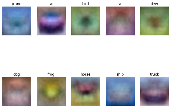
Another way to visually test the quality of the model is to visualize the model parameters. For example, if we identify the picture "horse", the model parameters are actually the picture "horse template", and the data can also be inferred through the visual parameters. For example, if there are a large number of pictures of "horse head left" and "horse head right", the trained model parameters are likely to become "double headed horse". Similarly, if most of the cars in the picture are red, the trained model may be a "red car template".
# Visually learned parameters
w = best_softmax.W[:-1,:] # Remove offset
w = w.reshape(32, 32, 3, 10)

w_min, w_max = np.min(w), np.max(w)

classes = ['plane', 'car', 'bird', 'cat', 'deer', 'dog', 'frog', 'horse', 'ship', 'truck']
for i in range(10):
    plt.subplot(2, 5, i + 1)
    #Scale the weight back to 0-255
    wimg = 255.0 * (w[:, :, :, i].squeeze() - w_min) / (w_max - w_min)
    plt.imshow(wimg.astype('uint8'))
    plt.axis('off')
    plt.title(classes[i])