1. Origin: GAN
Structure and principle
Before introducing DeblurGANv2, we need to know about GAN. GAN's initial application is image generation, that is, generating images according to the training set, such as handwritten digital images, face images, animal images, etc. its main structure is as follows:
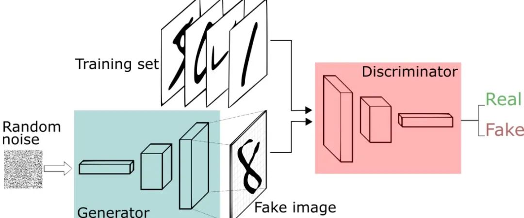
Let's start from the bottom left of the figure above. Assuming that there is only one sample now, that is, batch size is 1, then Random noise is a vector composed of random numbers subject to standard normal distribution. First, we input Random noise into the Generator. The Generator of the original GAN is a multi-layer perceptron. Its input is a vector and its output is also a vector. Then we reshape the output vector into a matrix, which is a picture (one matrix is because the pictures in MNIST handwritten data set are single channel gray-scale images. If you want to generate color images, reshape into three matrices), that is, it corresponds to "8" in the above figure. We call the image generated by Generator as fake image and the image in training set as real image.
The Discriminator in the figure above is a binary multi-layer perceptron that outputs only one number. Since the multi-layer perceptron only accepts vectors as its input, we expand a picture from a matrix into vectors and then input the Discriminator. After a series of operations, we output a number between 0 and 1. The closer this number is to 0, it means that the Discriminator thinks the picture is f Make image; on the contrary, if the output number is closer to 1, the Discriminator considers this picture as real image. For convenience, we abbreviate the Generator as G and the district as D.
In a word, G's purpose is to make its own generated fake image deceive D as much as possible, and D's task is to distinguish between fake image and real image as much as possible. In the end, ideally, the data generated by G is very close to the real data, and D outputs 0.5 regardless of whether it inputs fake image or real image.
loss function
The loss function of GAN is Binary cross entropy loss, abbreviated as BCELoss. It mainly uses the idea of maximum likelihood, which is actually the cross entropy loss function corresponding to binary classification. The formula is as follows:
Where is the number of samples, the real value of the first sample and the predicted value of the second sample. For the first sample, since the value can only be 0 or 1, only the first sample is looked at at at this time. At that time, the value range of,, is 0 ~ 1, so at that time, = 0. At that time, our goal is to make the smaller the value, the better, that is, when it is closer to 0, the smaller the value. On the contrary, at that time, the smaller the value Near 1, the smaller the value of. In short, the closer to, the smaller the value of.
So what is the relationship between BCELoss and GAN?
We divide the Loss of GAN into sum, that is, the Loss of generator and the Loss of discriminator.
-
For the generator, it hopes that the picture generated by itself can deceive the discriminator, that is, the closer D(fake) is to 1, the better. D(fake) is the output value of the picture generated by G after inputting D. D(fake) is close to 1, which means that the picture generated by G can deceive the discriminator with false and true. Therefore, the formula of GLoss is as follows:
When it is closer to 1, it is smaller, which means that the generator has cheated the discriminator;
-
For the discriminator, its loss is divided into two parts. First, it does not want to be deceived by the fake image, that is, on the contrary, it is represented here by:
The closer it is to 0, the smaller it is, which means that the discriminator recognizes the fake image;
Secondly, the judgment made by the discriminator must have a basis, so it needs to know what the real picture is to correctly distinguish the false picture, which is represented by:
When it is closer to 1, it is smaller, which means that the discriminator recognizes the real image.
In fact, it is the average of the two loss values:
optimizer
After introducing GAN's loss function, we still have one last question: how to make the value of the loss function smaller and smaller?
Here we need to talk about the Optimizer. The Optimizer is a tool to make the loss function value smaller and smaller. The commonly used optimizers include SGD, NAG, RMSProp, Adagrad, Adam and some variants of Adam, among which Adam is the most commonly used.
final result
It can be clearly seen from the above figure that with the increase of training rounds, the fake image generated by G is closer and closer to handwritten digits.
At present, GaN has many applications. For the corresponding papers and python codes of each application, please refer to the following links, including Gan codes. You can further understand Gan according to the codes: https://github.com/eriklindernoren/PyTorch-GAN
2. Image DeblurGANv2
data set
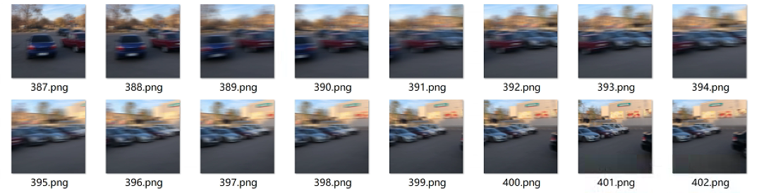
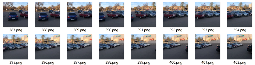
The data set of image deblurring is usually composed of many groups of images, and each group of images is a clear image and the corresponding blurred image. However, the production of its data set is not easy. At present, there are two commonly used methods: the first is to capture the video with a high frame number camera, and find the blurred pictures and clear pictures in consecutive frames from the video as a group of data; the second is The method is to use known or randomly generated motion blur to check clear pictures for blur operation and generate a corresponding set of data. Estimates is a commonly used data amplification Library in Python, which can rotate, zoom and crop pictures. We can also use estimates to add motion blur to images. The specific operations are as follows:
First, install the evaluations library, and enter in cmd or virtual environment:
python -m pip install albumentations
In order to add motion blur to the image, we need to use the matplotlib library to read, display and save the image.
import albumentations as A
from matplotlib import pyplot as plt
#  Reading and displaying the original drawing
img = plt.imread('./images/ywxd.jpg')
plt.imshow(img)
plt.axis('off')
plt.show()

Adding motion blur operations to augmentations is as follows, where blur_limit is the range of convolution kernel size, where the convolution kernel size is between 150 and 180. The larger the convolution kernel is, the more obvious the blur effect is; p is the probability of motion blur operation.
aug = A.MotionBlur(blur_limit=(50, 80), p=1.0)
aug_img = aug(image=img)['image']
plt.imshow(aug_img)
plt.axis('off')
plt.show()
If you want to view the corresponding fuzzy kernel, we can call the get_params method on the aug instance. Here, for your convenience, I use the 3 * 3 convolution kernel.
aug = A.MotionBlur(blur_limit=(3, 3), p=1.0)
aug.get_params()
{'kernel': array([[0.        , 0.        , 0.33333334],
       [0.33333334, 0.33333334, 0.        ],
       [0.        , 0.        , 0.        ]], dtype=float32)}
The dataset I use is DeblurGANv1, link: https://gas.graviti.cn/dataset/datawhale/BlurredSharp
Blurred picture:
Clear picture:
network structure
DeblurGANv2 has the same idea as GAN. The difference is that it optimizes GAN a lot. Let's first look at the structure of Generator:
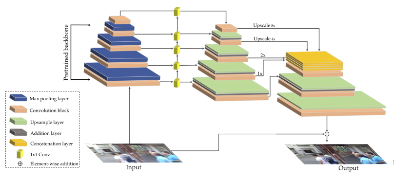
By observing the above figure, it can be found that G has two main changes:
-
The input replaces the random vector in GAN with a blurred picture
-
The network structure introduces FPN structure in target detection and integrates multi-scale features
In addition, in the feature extraction part, the author provides three network backbones: MobileNetv2, inception resnetv2 and densenet121. The author's experiment shows that inception resnetv2 has the best effect, but the model is large, while MobilNetv2 greatly reduces the network parameters without reducing too much effect. The corresponding part of the network backbone in the above figure is as follows:
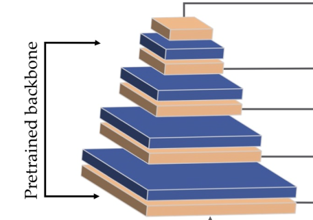
Finally, the output of fpn and the original image are added according to the elements to obtain the final output.
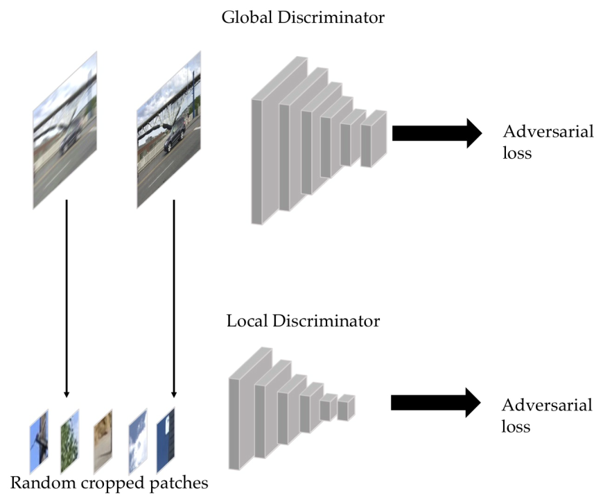
The discriminator of DeblurGANv2 consists of global and local parts. The global discriminator inputs the whole picture, and the local discriminator inputs the randomly cropped picture. After a series of convolution operations, the input picture outputs a number, which represents the probability that the discriminator considers it a real image. The structure of the discriminator is as follows:
loss function
The biggest difference between DeblurGANv2 and GAN is its loss function. Let's first look at D's loss:
The purpose of D is to distinguish the true and false of the picture. Therefore, when D(fake) is smaller and D(real) is larger, it means that D can well judge the true and false of the picture. Therefore, for D, the smaller the better
In order to prevent over fitting, an L2 penalty term will be added later:
G's loss is much more complex than D's. it consists of and. In fact, it is a perceptual loss. In fact, it inputs real image and fake image into vgg19 respectively, and makes the output characteristic map mselos (mean square error). The author has made some changes on the basis of perceptual loss. The formula can be summarized as follows:
It is easy to infer from the formula that the function of G is to make the image generated by G similar to the original image as much as possible to achieve the purpose of deblurring.
For, it can be summarized as the following formula:
Because the purpose of G is to deceive D as much as possible, the closer the sum is to 1, the better, that is, the smaller the sum is, the better.
Finally, the loss of G is as follows:
The lambda given by the author is 0.001, which shows that the author pays more attention to the similarity between the generated image and the original image.
3. Code practice
Train your own dataset
(currently only gpu training is supported!)
GitHub project address: https://github.com/VITA-Group/DeblurGANv2
Data address: https://gas.graviti.cn/dataset/datawhale/BlurredSharp
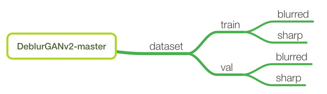
First, place the data folder and project folder according to the following structure:
Install the python environment and enter in cmd:
conda create -n deblur python=3.9
conda activate deblur
python -m pip install -r requirements.txt
Modify the configuration file config.yaml in the config folder:
project: deblur_gan
experiment_desc: fpn

train:
  files_a: &FILES_A ./dataset/train/blurred/*.png
  files_b: &FILES_B ./dataset/train/sharp/*.png
  size: &SIZE 256
  crop: random
  preload: &PRELOAD false
  preload_size: &PRELOAD_SIZE 0
  bounds: [0, .9]
  scope: geometric
  corrupt: &CORRUPT
    - name: cutout
      prob: 0.5
      num_holes: 3
      max_h_size: 25
      max_w_size: 25
    - name: jpeg
      quality_lower: 70
      quality_upper: 90
    - name: motion_blur
    - name: median_blur
    - name: gamma
    - name: rgb_shift
    - name: hsv_shift
    - name: sharpen

val:
  files_a: &FILE_A ./dataset/val/blurred/*.png
  files_b: &FILE_B ./dataset/val/sharp/*.png
  size: *SIZE
  scope: geometric
  crop: center
  preload: *PRELOAD
  preload_size: *PRELOAD_SIZE
  bounds: [.9, 1]
  corrupt: *CORRUPT

phase: train
warmup_num: 3
model:
  g_name: resnet
  blocks: 9
  d_name: double_gan # may be no_gan, patch_gan, double_gan, multi_scale
  d_layers: 3
  content_loss: perceptual
  adv_lambda: 0.001
  disc_loss: wgan-gp
  learn_residual: True
  norm_layer: instance
  dropout: True

num_epochs: 200
train_batches_per_epoch: 1000
val_batches_per_epoch: 100
batch_size: 1
image_size: [256, 256]

optimizer:
  name: adam
  lr: 0.0001
scheduler:
  name: linear
  start_epoch: 50
  min_lr: 0.0000001
If it is a windows system, you need to delete line 180 of train.py
Then cd to the project path in cmd and enter:
python train.py
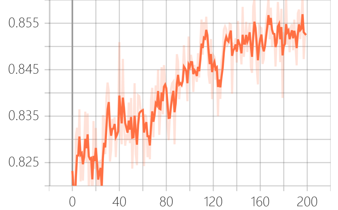
The training results can be visualized in tensorboard:
Verification set ssim (structural similarity):
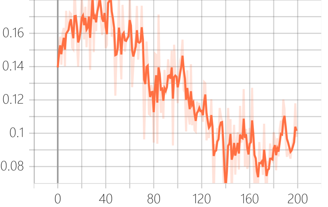
Validation set GLoss:
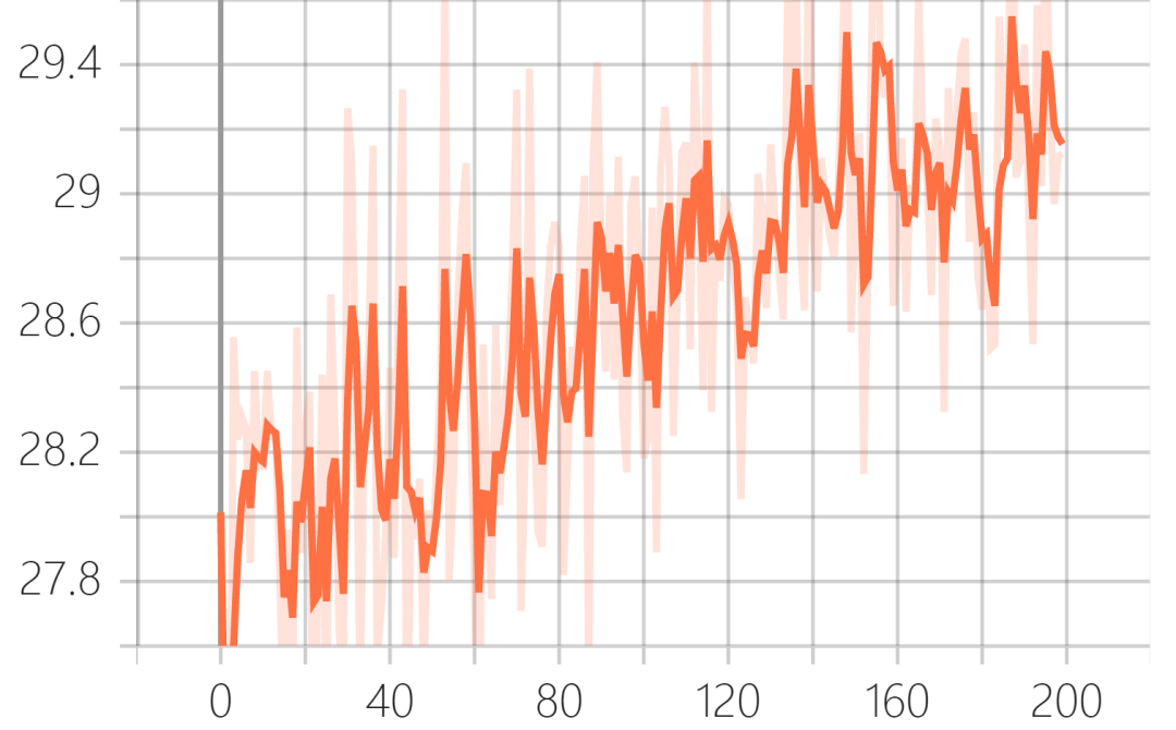
Verification set PSNR (peak signal-to-noise ratio):
Test (both CPU and GPU)
-
GPU
Save the test picture in test.png to deblurganv2 master folder, and enter in CMD:
python predict.py test.png
After successful operation, the model file in predict.py is best by default in the result submit folder_ Fpn.h5, you can also download the model file trained by the author in the github of DeblurGANv2, save it in the project folder, and change line 93 in the predict.py file to the model file you want to use, such as' best '_ Change FPN. H5 'to' fpn_inception.h5 ', but G corresponding to model in config.yaml_ Name is changed to the corresponding model. If you want to use 'fpn_mobilenet.h5 ', then' FPN_ Change 'inception' to 'FPN'_ mobilenet'
-
CPU
Change lines 21, 22 and 65 in the predict.py file to the following code
model.load_state_dict(torch.load(weights_path, map_location=torch.device('cpu'))['model'])
self.model = model
inputs = [img]
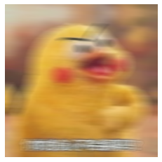
After running, you can get the following effects:


DeblurGAN's application: optimizing the performance of YOLOv5
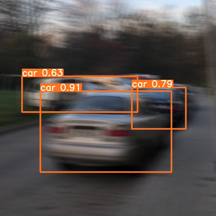
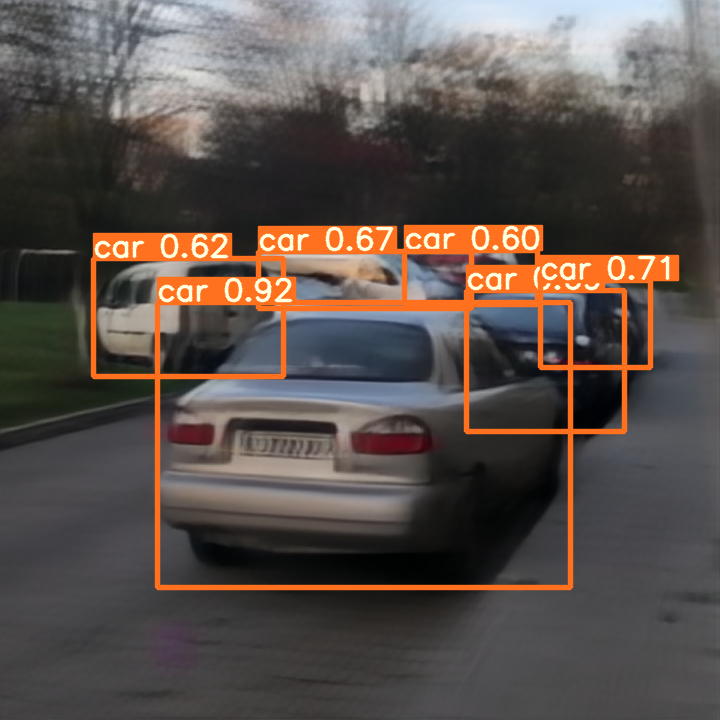
As can be seen from the above figure, image deblurring can not only improve the detection confidence of YOLOv5, but also make the detection more accurate. DeblurGANv2 with Mobilenetv2 as the backbone can meet the requirements of real-time image deblurring, and can be used in the direction of video quality enhancement.
Online training
If we don't want to download the data set locally, we can consider the online training function of Graviti and change a few lines of code on the basis of the original project.
First, open the dataset.py file in the project folder and import tensorbay and PIL in the first line (pip install is required if tensorbay is not installed):
from tensorbay import GAS
from tensorbay.dataset import Dataset as TensorBayDataset
from PIL import Image
We mainly modify the PairedDatasetOnline class and_ read_img function, in order to keep the original class, we can create a new class, copy and paste the following code into the dataset.py file (remember to change the ACCESS_KEY to the Graviti AccessKey of your own space):
class PairedDatasetOnline(Dataset):
    def __init__(self,
                 files_a: Tuple[str],
                 files_b: Tuple[str],
                 transform_fn: Callable,
                 normalize_fn: Callable,
                 corrupt_fn: Optional[Callable] = None,
                 preload: bool = True,
                 preload_size: Optional[int] = 0,
                 verbose=True):

        assert len(files_a) == len(files_b)

        self.preload = preload
        self.data_a = files_a
        self.data_b = files_b
        self.verbose = verbose
        self.corrupt_fn = corrupt_fn
        self.transform_fn = transform_fn
        self.normalize_fn = normalize_fn
        logger.info(f'Dataset has been created with {len(self.data_a)} samples')

        if preload:
            preload_fn = partial(self._bulk_preload, preload_size=preload_size)
            if files_a == files_b:
                self.data_a = self.data_b = preload_fn(self.data_a)
            else:
                self.data_a, self.data_b = map(preload_fn, (self.data_a, self.data_b))
            self.preload = True

    def _bulk_preload(self, data: Iterable[str], preload_size: int):
        jobs = [delayed(self._preload)(x, preload_size=preload_size) for x in data]
        jobs = tqdm(jobs, desc='preloading images', disable=not self.verbose)
        return Parallel(n_jobs=cpu_count(), backend='threading')(jobs)

    @staticmethod
    def _preload(x: str, preload_size: int):
        img = _read_img(x)
        if preload_size:
            h, w, *_ = img.shape
            h_scale = preload_size / h
            w_scale = preload_size / w
            scale = max(h_scale, w_scale)
            img = cv2.resize(img, fx=scale, fy=scale, dsize=None)
            assert min(img.shape[:2]) >= preload_size, f'weird img shape: {img.shape}'
        return img

    def _preprocess(self, img, res):
        def transpose(x):
            return np.transpose(x, (2, 0, 1))

        return map(transpose, self.normalize_fn(img, res))

    def __len__(self):
        return len(self.data_a)

    def __getitem__(self, idx):
        a, b = self.data_a[idx], self.data_b[idx]
        if not self.preload:
            a, b = map(_read_img, (a, b))
        a, b = self.transform_fn(a, b)
        if self.corrupt_fn is not None:
            a = self.corrupt_fn(a)
        a, b = self._preprocess(a, b)
        return {'a': a, 'b': b}

    @staticmethod
    def from_config(config):
        config = deepcopy(config)
        # files_a, files_b = map(lambda x: sorted(glob(config[x], recursive=True)), ('files_a', 'files_b'))
        segment_name = 'train' if 'train' in config['files_a'] else 'val'
        ACCESS_KEY = "yours"
        gas = GAS(ACCESS_KEY)
        dataset = TensorBayDataset("BlurredSharp", gas)
        segment = dataset[segment_name]
        files_a = [i for i in segment if 'blurred' == i.path.split('/')[2]]
        files_b = [i for i in segment if 'sharp' == i.path.split('/')[2]]
        transform_fn = aug.get_transforms(size=config['size'], scope=config['scope'], crop=config['crop'])
        normalize_fn = aug.get_normalize()
        corrupt_fn = aug.get_corrupt_function(config['corrupt'])
        # ToDo: add more hash functions
        verbose = config.get('verbose', True)

        return PairedDatasetOnline(files_a=files_a,
                             files_b=files_b,
                             preload=config['preload'],
                             preload_size=config['preload_size'],
                             corrupt_fn=corrupt_fn,
                             normalize_fn=normalize_fn,
                             transform_fn=transform_fn,
                             verbose=verbose)
Again_ read_ Change img to:
def _read_img(x):
    with x.open() as fp:
        img = cv2.cvtColor(np.asarray(Image.open(fp)), cv2.COLOR_RGB2BGR)
    if img is None:
        logger.warning(f'Can not read image {x} with OpenCV, switching to scikit-image')
        img = imread(x)[:, :, ::-1]
    return img
Finally, change the datasets = map(PairedDataset.from_config, datasets) in line 184 of train.py to datasets = map(PairedDatasetOnline.from_config, datasets).