1. Introduction to Matplotlib

Matplotlib is a Python 2D drawing library that can generate publication quality data in various hard copy formats and cross platform interactive environments. Matplotlib can be used for Python scripts, Python and IPython shell s, Jupyter notebooks, Web application servers, and four GUI toolkits.

2. matplotlib installation

matplotlib installation can use source installation and pip installation. Pip is installed as follows:

pip install matplotlib

Install the latest version by default, or install the specified version

pip install matplotlib==2.2.0

3. Maplotlib drawing example

3.1 common statistical graphs

• Scatter plot

x = np.arange(50)
y = x + 5 * np.random.rand(50)
plt.scatter(x, y)
plt.title('Scatter plot')                             # Add title
plt.xlabel('independent variable')                         # Add abscissa
plt.ylabel('dependent variable')                         # Add ordinate
plt.xlim(xmin=0, xmax=50)            # Add abscissa range 
plt.ylim(ymin=0, ymax=50)            # Add ordinate range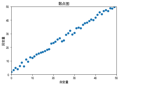

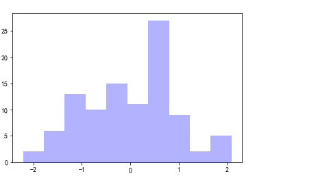
• histogram

  plt.hist(x=np.random.randn(100), bins=10, color='b', alpha=0.3)

  

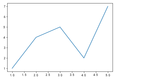
• Broken line diagram

  plt.plot([1,2,3,4,5],[1,4,5,2,7])

  

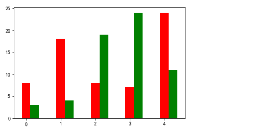
• Histogram

  x = np.arange(5)
  y1, y2 = np.random.randint(1, 25, size=(2, 5))
  width = 0.25
  plt.bar(x, y1, width, color='r')
  plt.bar(x+width, y2, width, color='g')

  

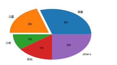
• Pie chart

explode=(0,0.1,0,0,0)
partions = [0.30,0.20,0.1,0.15,0.25]
labels = ['Apple','Samsung','millet','HUAWEI','others']
plt.pie(partions,labels=labels,explode=explode,autopct='%1.0f%%')

3.2 compilation of mathematical function curve

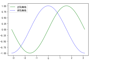
• trigonometric function

  x = np.arange(-np.pi,np.pi,0.01)
  y1 = np.sin(x)
  y2 = np.cos(x)
  plt.plot(x,y1,color='green',linewidth=1,linestyle='-',label='Sinusoidal curve')
  plt.plot(x,y2,color='blue',linewidth=1,linestyle='--',label='Cosine curve')
  plt.legend()   # Add annotation

  

• exponential function

  t = np.linspace(-50.0,50.0,1000)
  func_exp = np.exp(-0.1*t)
  plt.plot(t,func_exp)
  plt.title('exp(-0.1*t)')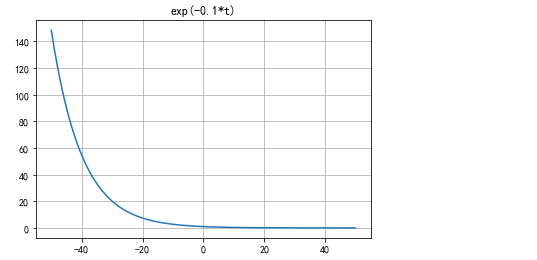

  

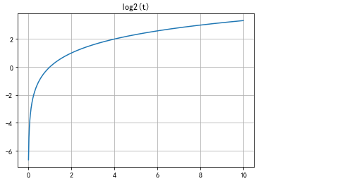
• Logarithmic function

  t = np.linspace(-10.0,10.0,1000)
  func_log2 = np.log2(t)
  plt.plot(t,func_log2)
  plt.title('log2(t)')
  plt.grid()