1. Concept of algorithm

Algorithm is the essence of computer processing information, because computer program is essentially an algorithm to tell the computer the exact steps to perform a specified task. Generally, when the algorithm is processing information, it will read the data from the input device or the storage address of the data, and write the result to the output device or a storage address for later call.

Algorithm is an independent method and idea to solve problems. For the algorithm, the language of implementation is not important, but the idea.

2. Five characteristics of the algorithm

1. Input: the algorithm has 0 or more inputs
2. Output: the algorithm has at least one or more outputs
3. Finiteness: the algorithm will automatically end after limited steps without infinite loop, and each step can be completed in an acceptable time
4. Certainty: every step in the algorithm has a definite meaning, and there will be no ambiguity
5. Feasibility: each step of the algorithm is feasible, that is, each step can be completed a limited number of times

3. Simple example of algorithm

If a+b+c=1000 and a2+b2=c^2 (a, b and c are natural numbers), how to find all possible combinations of a, b and c?
We use the enumeration method to solve this problem. As the name suggests, the enumeration method lists the answers one by one according to the requirements, and then judges whether to retain the answers according to the limiting conditions. Those that meet the requirements are retained and those that do not meet the requirements are discarded. Enumeration method is simple and rough, sometimes called violent solution method.

(1) Enumeration method I

import time

start_time = time.time()

# Note that it is a triple cycle
for a in range(0, 1001):
    for b in range(0, 1001):
        for c in range(0, 1001):
            if a**2 + b**2 == c**2 and a+b+c == 1000:
                print("a, b, c: %d, %d, %d" % (a, b, c))

end_time = time.time()
print("elapsed: %f" % (end_time - start_time))
print("complete!")

Execution results:
	a, b, c: 0, 500, 500
	a, b, c: 200, 375, 425
	a, b, c: 375, 200, 425
	a, b, c: 500, 0, 500
	elapsed: 214.583347
	complete!

(2) Enumeration method II

import time

start_time = time.time()

# Note that it is a double cycle
for a in range(0, 1001):
    for b in range(0, 1001-a):
        c = 1000 - a - b
        if a**2 + b**2 == c**2:
            print("a, b, c: %d, %d, %d" % (a, b, c))

end_time = time.time()
print("elapsed: %f" % (end_time - start_time))
print("complete!")

Execution results:
	a, b, c: 0, 500, 500
	a, b, c: 200, 375, 425
	a, b, c: 375, 200, 425
	a, b, c: 500, 0, 500
	elapsed: 0.182897
	complete!

Summary: for the same problem, the first method uses triple loop, and the running time for solving the problem is 214.58s, while the second method uses double loop, and the running time for solving the problem is 0.18s. It can be seen that the efficiency of solving the same problem will be different by using different algorithms. In essence, the algorithm time complexity of the first method is O(n^3), the algorithm time complexity of the second method is O(n ^2), and O(n^3) is greater than O(n ^2).

4. Measurement of algorithm efficiency

4.1 execution time response algorithm efficiency

For the same problem, we give two algorithms. In the implementation of the two algorithms, we calculate the execution time of the program and find that the execution time of the two programs is very different (214.583347 seconds compared with 0.182897 seconds). Therefore, we can draw a conclusion that the execution time of the program implementing the algorithm can reflect the efficiency of the algorithm, that is, the advantages and disadvantages of the algorithm.

4.2 time value alone is not absolutely credible

Suppose we run the algorithm program of the second attempt on a computer with old configuration and low performance? It is likely that the running time will not be much faster than the 214.583347 seconds of algorithm I running on our computer.

Simply relying on the running time to compare the advantages and disadvantages of the algorithm is not necessarily objective and accurate!

The running of the program is inseparable from the computer environment (including hardware and operating system). These objective reasons will affect the running speed of the program and reflect on the execution time of the program.

4.3 time complexity and "Big O notation"

Assuming that the time for the computer to perform each basic operation of the algorithm is a fixed time unit, how many basic operations represent how many time units it will take. However, for different machine environments, the exact unit time is different, but the number of basic operations (i.e. how many time units it takes) of the algorithm is the same in the order of magnitude. Therefore, the influence of the machine environment can be ignored and the time efficiency of the algorithm can be reflected objectively.

For the time efficiency of the algorithm, we can use "Big O notation":

"Large o notation": for monotonic integer function f, if there is an integer function g and real constant C > 0, so that for sufficiently large N, there is always f (n) < = C * g (n), that is, function g is an asymptotic function of F (ignoring the constant), which is recorded as f(n)=O(g(n)). In other words, in the sense of the limit towards infinity, the growth rate of function f is constrained by function g, that is, the characteristics of function f and function g are similar.

Time complexity: assuming that there is A function g such that the time taken by algorithm A to process the problem example with scale n is T(n)=O(g(n)), then O(g(n)) is called the asymptotic time complexity of algorithm A, referred to as time complexity for short, and recorded as T(n).

4.4 understand "Big O notation"

Although it is good to analyze the algorithm in detail, it has limited practical value in practice. For the temporal and spatial properties of the algorithm, the most important is its order of magnitude and trend, which are the main parts of analyzing the efficiency of the algorithm. The constant factors in the scale function of the basic operation quantity of the measurement algorithm can be ignored. For example, it can be considered that 3n^2 and 100n ^2 belong to the same order of magnitude. If the cost of the two algorithms for processing instances of the same size is these two functions respectively, their efficiency is considered to be "almost" and both are n ^2.

4.5 worst time complexity

There are several possible considerations when analyzing the algorithm:

(1) How many basic operations does the algorithm need to complete the work, that is, the optimal time complexity
(2) How many basic operations does the algorithm need to complete the work, that is, the worst time complexity
(3) The average number of basic operations required for the algorithm to complete the work, that is, the average time complexity

[1] For the optimal time complexity, it is of little value because it does not provide any useful information. It only reflects the most optimistic and ideal situation, and has no reference value.
[2] For the worst time complexity, it provides a guarantee that the algorithm can complete the work in this level of basic operation.
[3] The average time complexity is a comprehensive evaluation of the algorithm, so it completely reflects the properties of the algorithm. On the other hand, there is no guarantee that not every calculation can be completed within this basic operation. Moreover, it is difficult to calculate the average case because the instance distribution of the application algorithm may not be uniform.

Therefore, we mainly focus on the worst case of the algorithm, that is, the worst time complexity.

4.6 several basic calculation rules of time complexity

(1) The basic operation, that is, there is only a constant term, is considered to have a time complexity of O(1)
(2) Sequential structure, and the time complexity is calculated by addition
(3) Loop structure, and the time complexity is calculated by multiplication
(4) Branching structure, the time complexity is the maximum
(5) When judging the efficiency of an algorithm, we often only need to pay attention to the highest order term of the number of operations, and other secondary terms and constant terms can be ignored. In the absence of special instructions, the time complexity of the algorithm we analyze refers to the worst time complexity.

5. Common time complexity analysis

Example of execution times function	rank	informal term
12	O(1)	Constant order
2n+3	O(n)	Linear order
3n2+2n+1	O(n2)	Square order
5log2n+20	O(logn)	Logarithmic order
2n+3nlog2n+19	O(nlogn)	nlogn order
6n3+2n2+3n+4	O(n3)	Cubic order
2n	O(2n)	Exponential order

Note: log2n (logarithm based on 2) is generally abbreviated as logn

Combined with image understanding:

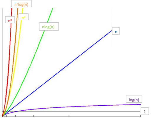
Comparison of elapsed time:

O(1) < O(logn) < O(n) < O(nlogn) < O(n^ 2) < O(n ^3) < O(2 ^n) < O(n!) < O(n ^n)

6.Python built-in type performance analysis

6.1 timeit module

The timeit module can be used to test the execution speed of a small piece of Python code.

class timeit.Timer(stmt='pass', setup='pass', timer=)
(1) Timer is a class that measures the execution speed of small pieces of code.

(2) stmt parameter is the code statement to be tested;

(3) The setup parameter is the setting required to run the code;

(4) The timer parameter is a timer function, which is platform related.

timeit.Timer.timeit(number=1000000)
The object method in the Timer class that tests the execution speed of statements. The number parameter is the number of tests when testing the code. The default is 1000000. Method returns the average time spent executing code, in seconds of a float type.

6.1 operation test of list

def test1():
   l = []
   for i in range(1000):
      l = l + [i]
def test2():
   l = []
   for i in range(1000):
      l.append(i)
def test3():
   l = [i for i in range(1000)]
def test4():
   l = list(range(1000))

from timeit import Timer

t1 = Timer("test1()", "from __main__ import test1")
print("concat ",t1.timeit(number=1000), "seconds")
t2 = Timer("test2()", "from __main__ import test2")
print("append ",t2.timeit(number=1000), "seconds")
t3 = Timer("test3()", "from __main__ import test3")
print("comprehension ",t3.timeit(number=1000), "seconds")
t4 = Timer("test4()", "from __main__ import test4")
print("list range ",t4.timeit(number=1000), "seconds")

Execution results:
	# ('concat ', 1.7890608310699463, 'seconds')
	# ('append ', 0.13796091079711914, 'seconds')
	# ('comprehension ', 0.05671119689941406, 'seconds')
	# ('list range ', 0.014147043228149414, 'seconds')

pop operation test

x = range(2000000)
pop_zero = Timer("x.pop(0)","from __main__ import x")
print("pop_zero ",pop_zero.timeit(number=1000), "seconds")
x = range(2000000)
pop_end = Timer("x.pop()","from __main__ import x")
print("pop_end ",pop_end.timeit(number=1000), "seconds")

Execution results:
	# ('pop_zero ', 1.9101738929748535, 'seconds')
	# ('pop_end ', 0.00023603439331054688, 'seconds')

Test pop operation: it can be seen from the results that the efficiency of the last element of pop is much higher than that of the first element of pop

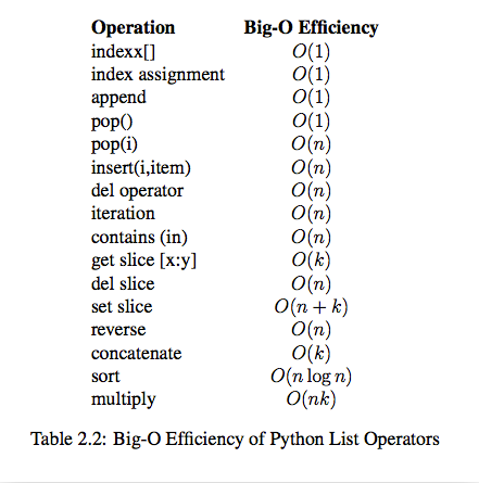
6.2 time complexity of list built-in operation

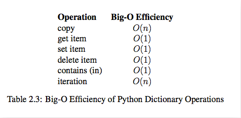
6.3 time complexity of built-in operation of Dict