1. Group by a column to determine whether there are duplicate columns.
# Count the unique variables (if we got different weight values,
# for example, then we should get more than one unique value in this groupby)
all_cols_unique_players = df.groupby('playerShort').agg({col:'nunique' for col in player_cols})
For the. agg function:
DataFrame.agg(self, func, axis=0, *args, **kwargs)[source]
Aggregate using one or more operations over the specified axis.
Example:
>>> df = pd.DataFrame([[1, 2, 3],
...                    [4, 5, 6],
...                    [7, 8, 9],
...                    [np.nan, np.nan, np.nan]],
...                   columns=['A', 'B', 'C'])


>>> df.agg({'A' : ['sum', 'min'], 'B' : ['min', 'max']})
        A    B
max   NaN  8.0
min   1.0  2.0
sum  12.0  NaN
2. Get a word list
"Helper function that creates a sub table from the columns and runs a quick uniformity test." "
player_index = 'playerShort'
player_cols = [#'player', # drop player name, we have unique identifier
               'birthday',
               'height',
               'weight',
               'position',
               'photoID',
               'rater1',
               'rater2',
              ]
def get_subgroup(dataframe, g_index, g_columns):
    """Helper function that creates a sub-table from the columns and runs a quick uniqueness test."""
    g = dataframe.groupby(g_index).agg({col:'nunique' for col in g_columns})
    if g[g > 1].dropna().shape[0] != 0:
        print("Warning: you probably assumed this had all unique values but it doesn't.")
    return dataframe.groupby(g_index).agg({col:'max' for col in g_columns})
players = get_subgroup(df, player_index, player_cols)
players.head()
3. Save the sorted word table to CSV file
def save_subgroup(dataframe, g_index, subgroup_name, prefix='raw_'):
    save_subgroup_filename = "".join([prefix, subgroup_name, ".csv.gz"])
    dataframe.to_csv(save_subgroup_filename, compression='gzip', encoding='UTF-8')
    test_df = pd.read_csv(save_subgroup_filename, compression='gzip', index_col=g_index, encoding='UTF-8')
    # Test that we recover what we send in
    if dataframe.equals(test_df):
        print("Test-passed: we recover the equivalent subgroup dataframe.")
    else:
        print("Warning -- equivalence test!!! Double-check.")
4. View specific data indicators - view missing values
import missingno as msno
import pandas_profiling
msno.matrix(players.sample(500),
            figsize=(16, 7),
            width_ratios=(15, 1))
msno.heatmap(players.sample(500),
            figsize=(16, 7),)

5. PivotTable
Go to https://blog.csdn.net/dorisi'h'n'q/article/details/82288092
Pivot table concept: PD. Pivot table()
Pivot table is a common data summary tool in various spreadsheet programs and other data analysis software. It aggregates data based on one or more keys and allocates data to rectangular areas based on grouping keys on rows and columns.
 Pivot table: group calculation according to specific conditions, find data, and calculate
pd.pivot_table(df,index=['hand'],columns=['male'],aggfunc='min')
Concept of crosstab: pd.crosstab (index, colors)
Crosstab is a special perspective used to calculate grouping frequency and summarize data.
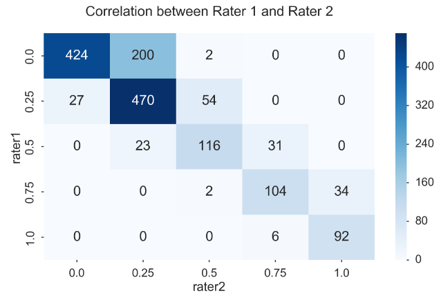
pd.crosstab(players.rater1, players.rater2)
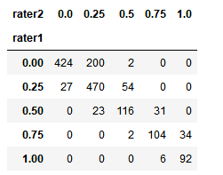
fig, ax = plt.subplots(figsize=(12, 8))
sns.heatmap(pd.crosstab(players.rater1, players.rater2), cmap='Blues', annot=True, fmt='d', ax=ax)
ax.set_title("Correlation between Rater 1 and Rater 2\n")
fig.tight_layout()
Create a new column whose value is the average of the other two columns
players['skintone'] = players[['rater1', 'rater2']].mean(axis=1)
players.head()
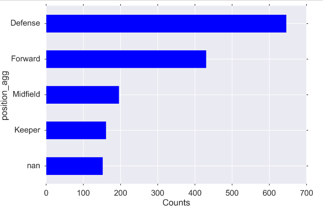
6. Process the discrete category value
(Create higher level categories)
position_types = players.position.unique()
position_types
"""
array(['Center Back', 'Attacking Midfielder', 'Right Midfielder',
       'Center Midfielder', 'Goalkeeper', 'Defensive Midfielder',
       'Left Fullback', nan, 'Left Midfielder', 'Right Fullback',
       'Center Forward', 'Left Winger', 'Right Winger'], dtype=object)
"""

defense = ['Center Back','Defensive Midfielder', 'Left Fullback', 'Right Fullback', ]
midfield = ['Right Midfielder', 'Center Midfielder', 'Left Midfielder',]
forward = ['Attacking Midfielder', 'Left Winger', 'Right Winger', 'Center Forward']
keeper = 'Goalkeeper'

# modifying dataframe -- adding the aggregated position categorical position_agg
players.loc[players['position'].isin(defense), 'position_agg'] = "Defense"
players.loc[players['position'].isin(midfield), 'position_agg'] = "Midfield"
players.loc[players['position'].isin(forward), 'position_agg'] = "Forward"
players.loc[players['position'].eq(keeper), 'position_agg'] = "Keeper"
Draw a value_counts() picture
MIDSIZE = (12, 8)
fig, ax = plt.subplots(figsize=MIDSIZE)
players['position_agg'].value_counts(dropna=False, ascending=True).plot(kind='barh', ax=ax)
ax.set_ylabel("position_agg")
ax.set_xlabel("Counts")
fig.tight_layout()
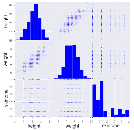
7. Draw the relationship between variables
from pandas.plotting import scatter_matrix
fig, ax = plt.subplots(figsize=(10, 10))
scatter_matrix(players[['height', 'weight', 'skintone']], alpha=0.2, diagonal='hist', ax=ax);
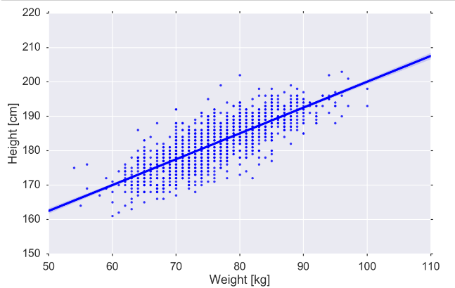
# Perhaps you want to see a particular relationship more clearly
fig, ax = plt.subplots(figsize=MIDSIZE)
sns.regplot('weight', 'height', data=players, ax=ax)
ax.set_ylabel("Height [cm]")
ax.set_xlabel("Weight [kg]")
fig.tight_layout()
8. Create quantitative bins for continuous variables
weight_categories = ["vlow_weight",
                     "low_weight",
                     "mid_weight",
                     "high_weight",
                     "vhigh_weight",
                    ]

players['weightclass'] = pd.qcut(players['weight'],
                                 len(weight_categories),
                                 weight_categories)
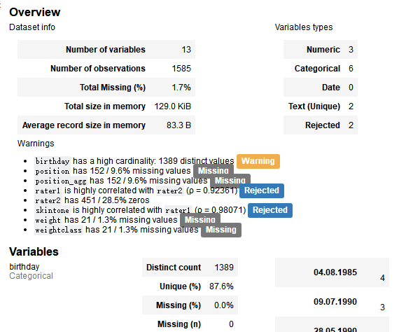
9. View data report
pandas_profiling.ProfileReport(players)
10. Time format processing such as birth date
players['birth_date'] = pd.to_datetime(players.birthday, format='%d.%m.%Y')
players['age_years'] = ((pd.to_datetime("2013-01-01") - players['birth_date']).dt.days)/365.25
players['age_years']
//Select a specific column
players_cleaned_variables = players.columns.tolist()
players_cleaned_variables
player_dyad = (clean_players.merge(agg_dyads.reset_index().set_index('playerShort'),
                                   left_index=True,
                                   right_index=True))
//groupby+sort_values+rename
(tidy_dyads.groupby(level=1)
           .sum()
           .sort_values('redcard', ascending=False)
           .rename(columns={'redcard':'total redcards received'})).head()