Because different dimensions may affect the observation results of data

Solution: Map all data to the same scale

1. Maximum Normalization: Mapping all data to 0-1

Suitable for situations with clear boundaries, greatly influenced by Outlier

xscale=x−xmin⁡xmax⁡−xmin⁡x_{\text {scale}}=\frac{x-x_{\min }}{x_{\max }-x_{\min }}xscale​=xmax​−xmin​x−xmin​​

2. Standardization of mean variance:
Normalize all data into data with a mean of 0 and a variance of 1

It can be applied to situations where there are no obvious boundaries of data and there may be extreme data values. It also applies to cases where data have obvious boundaries.

xscale=x−xmeansx_{s c a l e}=\frac{x-x_{m e a n}}{s}xscale​=sx−xmean​​

Code example: (written in jupyter notebook)

1. Data normalization

import numpy as np
import matplotlib.pyplot as plt

Maximum Normalization

x = np.random.randint(0, 100, size=100) # 0 to 100 vectors, a total of 100
x

The result is:

array([29, 19, 31, 31, 9, 59, 14, 76, 69, 34, 30, 97, 13, 96, 0, 52,
86, 96, 40, 39, 98, 70, 76, 84, 82, 95, 52, 94, 84, 59, 89, 11, 29, 2,
99, 69, 44, 48, 48, 92, 54, 46, 1, 43, 16, 52, 51, 26, 83, 94, 50,74, 55, 30, 18, 44, 36, 62, 8, 56, 12, 44, 27, 26, 43, 88, 86, 58,12, 39, 62, 31, 77, 23, 78, 0, 58, 97, 58, 38, 83, 56, 70, 72, 84,54, 75, 2, 71, 1, 84, 77, 5, 23, 50, 3, 1, 58, 74, 47])

(x-np.min(x))/(np.max(x)-np.min(x)) # Maximum Normalization

The result is:

array([0.95918367, 0.59183673, 0.92857143, 0.85714286, 0.34693878, 0.97959184, 0.63265306, 0.05102041, 0.09183673, 0.47959184, 0.69387755, 0.30612245, 0.09183673, 0.85714286, 0.21428571, 0.23469388, 0.90816327, 0. , 0.73469388, 0.90816327, 0.36734694, 0.69387755, 0.2755102 , 0.45918367, 0.56122449, 0.21428571, 0.31632653, 0.85714286, 0.64285714, 0.26530612, 0.41836735, 0.90816327, 1. , 0.82653061, 0.16326531, 0.10204082, 0.6122449 , 0.87755102, 0.03061224, 0.2244898 , 0.48979592, 0.56122449, 0.33673469, 0.8877551 , 0.74489796, 0.01020408, 0.89795918, 0.89795918, 0.12244898, 0.41836735, 0.24489796, 0.18367347, 0.59183673, 0.51020408, 0.26530612, 0.59183673, 0.81632653, 0.07142857, 0.42857143, 0.8877551 , 0.04081633, 0.6122449 , 0.3877551 , 0.92857143, 0.70408163, 0.67346939, 0.20408163, 0.30612245, 0.87755102, 0.87755102, 0.60204082, 0.86734694, 0.19387755, 0.02040816, 0.39795918, 0.83673469, 0.02040816, 0.94897959, 0.23469388, 0.16326531, 0.26530612, 0.48979592, 0.20408163, 1. , 0.04081633, 0.42857143, 0.87755102, 0.20408163, 0.04081633, 0.21428571, 0.79591837, 0.17346939, 0.43877551, 0.21428571, 0.54081633, 0.83673469, 0.79591837, 0.17346939, 0.70408163, 0.79591837])

x = np.random.randint(0, 100, (50, 2)) # A matrix of 50*2 dimensions, with values ranging from 0 to 100

x[:10, :] # Take the top 10 elements

The result is:

array([[80, 95],
[ 1, 70],
[18, 70],
[31, 86],
[48, 57],
[84, 68],
[90, 29],
[44, 60],
[18, 39],
[42, 55]])

x = np.array(x, dtype=float) # Convert to floating point number

x[:10, :]

The result is:

array([[80., 95.],
[ 1., 70.],
[18., 70.],
[31., 86.],
[48., 57.],
[84., 68.],
[90., 29.],
[44., 60.],
[18., 39.],
[42., 55.]])

x[:, 0] = (x[:, 0] - np.min(x[:, 0]))/(np.max(x[:, 0]) - np.min(x[:,
0])) # For column 0 (the first feature), normalize x [:, 1]= (x [:, 1] - np. min (x [:, 1],
1]))/(np.max(x[:, 1]) - np.min(x[:, 1])) # Maximum normalization of column 1 (second feature)

x[:10, :]

The result is:

array([[0.84210526, 0.96938776],
[0.01052632, 0.71428571],
[0.18947368, 0.71428571],
[0.32631579, 0.87755102],
[0.50526316, 0.58163265],
[0.88421053, 0.69387755],
[0.94736842, 0.29591837],
[0.46315789, 0.6122449 ],
[0.18947368, 0.39795918],
[0.44210526, 0.56122449]])

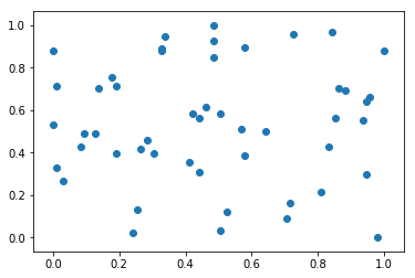
plt.scatter(x[:, 0], x[:, 1])
plt.show()

np.mean(x[:, 0]) # Means corresponding to column 0

The result is:
0.4785263157894737

np.std(x[:, 0]) # Variance corresponding to column 0

The result is:
0.3047560942923213

np.mean(x[:, 1]) # Means corresponding to column 1

The result is:
0.5375510204081633

np.std(x[:, 1]) # Variance corresponding to column 1

The result is:
0.2753547558441912

2. Standardization of Mean Variance Normalization

x2 = np.random.randint(0, 100, (50, 2)) # matrix

x2 = np.array(x2, dtype=float) # Converting to floating-point type

x2[:, 0] = (x2[:, 0] - np.mean(x2[:, 0]))/ np.std(x2[:, 0]) # Normalization of Mean Variance in Column 0

x2[:, 1] = (x2[:, 1] - np.mean(x2[:, 1]))/ np.std(x2[:, 1]) # Normalization of mean variance in column 1

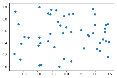
plt.scatter(x2[:, 0], x[:, 1])
plt.show()

np.mean(x2[:, 0]) # Means corresponding to column 0

The result is:
-2.2204460492503132e-17

np.std(x2[:, 0]) # Variance corresponding to column 0

The result is:
0.9999999999999998

np.mean(x2[:, 1]) # Means corresponding to column 1

The result is:
-7.549516567451065e-17

np.std(x2[:, 1]) # Variance corresponding to column 1

The result is:
0.9999999999999999