This blog is a reading note of "data analysis by Python". Please do not reprint it for other business purposes.
Article directory
1. Hierarchical index
Hierarchical index is an important feature of pandas, which allows you to have more than one (two or more) index level in another axis. Generally speaking, hierarchical index provides a way to process higher dimension data in the form of lower dimension. Example:
data = pd.Series(np.random.randn(9),
                index=[['a', 'a', 'a', 'b', 'b', 'c', 'c', 'd', 'd'],
                [1, 2, 3, 1, 3, 1, 2, 2, 3]])
data
#
a  1    0.084340
   2    1.252705
   3   -1.305060
b  1    0.629035
   3   -1.099427
c  1   -0.785977
   2   -0.524298
d  2    0.144326
   3    0.945895
dtype: float64
What we see is a fancy view of a Series indexed by MultiIndex. The "gap" in the index means "use the above label directly":
data.index
#
MultiIndex(levels=[['a', 'b', 'c', 'd'], [1, 2, 3]],
           codes=[[0, 0, 0, 1, 1, 2, 2, 3, 3], [0, 1, 2, 0, 2, 0, 1, 1, 2]])
Through layered index objects, they can also be partial indexes, allowing you to select a subset of data concisely:
data['b']
#
1    0.629035
3   -1.099427
dtype: float64
data['b': 'c']
#
b  1    0.629035
   3   -1.099427
c  1   -0.785977
   2   -0.524298
dtype: float64
data.loc[['b', 'd']]
#
b  1    0.629035
   3   -1.099427
d  2    0.144326
   3    0.945895
dtype: float64
It is also possible to choose at the internal level:
data.loc[:, 2]
#
a    1.252705
c   -0.524298
d    0.144326
dtype: float64
Hierarchical index plays an important role in grouping operations such as reshaping data and array PivotTable. For example, you can use the unstack method to rearrange data in a DataFrame:
data.unstack()
#
            1	        2	        3
a	 0.084340	 1.252705	-1.305060
b	 0.629035	      NaN	-1.099427
c	-0.785977	-0.524298	      NaN
d	      NaN	 0.144326	 0.945895
The counter operation of unstack is stack:
data.unstack().stack()
#
a  1    0.084340
   2    1.252705
   3   -1.305060
b  1    0.629035
   3   -1.099427
c  1   -0.785977
   2   -0.524298
d  2    0.144326
   3    0.945895
dtype: float64
In DataFrame, each axis can have a hierarchical index:
frame = pd.DataFrame(np.arange(12).reshape((4, 3)),
                    index=[['a', 'a', 'b', 'b'], [1, 2, 1, 2]],
                    columns=[['Ohio', 'Ohio', 'Colorado'],
                            ['Green', 'Red', 'Green']])
frame
#
      Ohio	 Colorado
     Green	Red	Green
a	1	 0	  1	    2
    2	 3	  4	    5
b	1	 6	  7	    8
    2	 9	 10    11
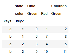
A hierarchical level can have names (can be strings or Python objects). If the hierarchy has names, they are displayed in the console output:
frame.index.names = ['key1', 'key2']
frame.columns.names = ['state', 'color']
frame
#
state	Ohio	Colorado
color	Green	Red	Green
key1 key2
a	 1	    0	  1	    2
     2	    3	  4	    5
b	 1	    6	  7	    8
     2   	9    10	   11
Note the index names' state 'and' color 'in the area line label.
With a partial column index, you can select groups in the columns:
frame['Ohio']
#
color	Green	Red
key1 key2
a	 1	    0	  1
     2  	3     4
b	 1	    6	  7
     2	    9	 10
1.1 reorder and hierarchy
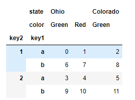
Sometimes, we need to reorder the hierarchy on the axis, or sort the data according to the value of a specific hierarchy. swaplevel receives two level serial numbers or level names, and returns a new object with level changes (but the data is unchanged):
frame.swaplevel('key1', 'key2')
#
state	Ohio	Colorado
color	Green	Red	Green
key1 key2
a	 1	    0	  1	    2
     2	    3	  4	    5
b	 1	    6	  7	    8
     2   	9    10	   11
On the other hand, sort ® index can only sort data at a single level. When performing hierarchical transformation, it is also common to use sort ﹣ index to sort the dictionary according to the hierarchy based on the result of yes:
frame.sort_index(level=1)
frame.swaplevel(0, 1).sort_index(level=0)
If the indexes are sorted from the outermost layer in dictionary order, data selection performance will be better -- such results can be obtained by calling sort_index(level=0) or sort_index.
1.2 summary statistics by level
Usually we don't use one or more columns in the DataFrame as row indexes; instead, you may want to move row indexes to columns in the DataFrame. Here is an example:
frame = pd.DataFrame({'a': range(7), 'b': range(7, 0, -1),
                      'c': ['one', 'one', 'one', 'two', 'two',
                            'two', 'two'],
                      'd': [0, 1, 2, 0, 1, 2, 3]})
frame
#
   a  b    c  d
0  0  7  one  0
1  1  6  one  1
2  2  5  one  2
3  3  4  two  0
4  4  3  two  1
5  5  2  two  2
6  6  1  two  3
The set ﹣ index function of DataFrame will generate a new DataFrame, which uses one or more columns as the index:
frame2 = frame.set_index(['c', 'd'])
frame2
#
       a  b
c   d
one 0  0  7
    1  1  6
    2  2  5
two 0  3  4
    1  4  3
    2  5  2
    3  6  1
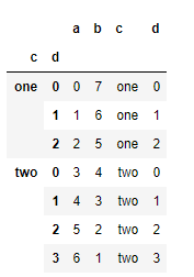
By default, these columns are removed from the DataFrame, and you can also leave them in the DataFrame:
frame.set_index(['c', 'd'], drop=False)
#
On the other hand, reset index is the reverse operation of set index. The index level of the hierarchical index will be moved to the column: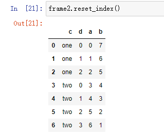
2. Join and merge datasets
Data contained in pandas objects can be combined in many ways:
- pandas.merge connects rows based on one or more keys. For users of SQL or other relational databases, this method is quite familiar. It implements the connection operation of the database.
- pandas.concat causes objects to glue or "stack" axially.
- The combine first instance method allows overlapping data to be spliced together to fill in missing values in an object with values from an object.
2.1 database style DataFrame connection
A merge or join operation joins a dataset by joining rows with one or more keys. These operations are the core content of relational databases (such as SQL based databases). The merge function in panda is mainly used to apply various join operation algorithms to data:
df1 = pd.DataFrame({'key': ['b', 'b', 'a', 'c', 'a', 'a', 'b'],
                    'data1': range(7)})
df2 = pd.DataFrame({'key': ['a', 'b', 'd'],
                     'data2': range(3)})
df1
#
  key	data1
0	b	0
1	b	1
2	a	2
3	c	3
4	a	4
5	a	5
6	b	6

df2
#
  key	data2
0	a	0
1	b	1
2	d	2
This is a many to one example; df1 data has multiple rows labeled a and b, while df2 has only one row for each value in the key column. Call merge to process the object we get:
pd.merge(df1, df2)
#
	key	data1	data2
0	  b	    0	    1
1	  b	    1	    1
2	  b	    6	    1
3	  a	    2	    0
4	  a	    4	    0
5	  a	    5	    0
Note that we did not specify which column to join on. If the key information of the connection is not specified, merge will automatically use the overlapping column name as the key of the connection. However, specifying the connection key explicitly is a good implementation:
pd.merge(df1, df2, on='key')
The result is the same as before.
If the column names of each object are different, you can specify them separately:
df3 = pd.DataFrame({'lkey': ['b', 'b', 'a', 'c', 'a', 'a', 'b'],
                    'data1': range(7)})
df4 = pd.DataFrame({'rkey': ['a', 'b', 'd'],
                     'data2': range(3)})
pd.merge(df3, df4, left_on='lkey', right_on='rkey')
#
  lkey	data1	rkey	data2
0	 b	    0	   b	    1
1	 b	    1	   b	    1
2	 b	    6	   b	    1
3	 a	    2	   a	    0
4	 a	    4	   a	    0
5	 a	    5	   a	    0
We can find that the results are lack of 'c' and 'd' values and related data. By default, merge does inner join, and the key in the result is the intersection of two tables. Other options are 'left', 'right' and 'outer'. External connection is the intersection of keys, combining the effects of left connection and right connection:
pd.merge(df1, df2, how='outer')
#
  key	data1	data2
0	b	  0.0	  1.0
1	b	  1.0	  1.0
2	b	  6.0	  1.0
3	a	  2.0	  0.0
4	a	  4.0	  0.0
5	a	  5.0	  0.0
6	c	  3.0	  NaN
7	d	  NaN	  2.0
Table: different connection types of how parameters
| option | behavior |
|---|---|
| inner | Join only the intersection of keys in both tables |
| left | Union keys for all left tables |
| right | Union keys of all right tables |
| outer | Union of union of keys in both tables |
Although it is not very intuitive, many to many merging has a clear behavior. Here is an example:
df1 = pd.DataFrame({'key': ['b', 'b', 'a', 'c', 'a', 'a', 'b'],
                    'data1': range(7)})
df2 = pd.DataFrame({'key': ['a', 'b', 'd'],
                     'data2': range(3)})
df1
#
  key data1
0	b	  0
1	b	  1
2	a	  2
3	c	  3
4	a	  4
5	a	  5
6	b	  6
df2
#
  key	data2
0	a	    0
1	b	    1
2	d	    2
pd.merge(df1, df2)
#
  key	data1	data2
0	b	    0	    1
1	b	    1	    1
2	b	    6	    1
3	a	    2	    0
4	a	    4	    0
5	a	    5 	    0
Many to many connections are Cartesian products of rows. Since there are three 'b' rows in the DataFrame on the left and two on the right, there are six 'b' rows in the result. The connection method only affects the different key values displayed in the result:
pd.merge(df1, df2, on='key')
#
  key	data1	data2
0	b	    0	    1
1	b	    1	    1
2	b	    6	    1
3	a	    2	    0
4	a	    4	    0
5	a	    5	    0
When merging with multiple keys, pass in a list of column names:
left = pd.DataFrame({'key1': ['foo', 'foo', 'bar'],
                     'key2': ['one', 'two', 'one'],
                     'lval':[1, 2, 3]})
right = pd.DataFrame({'key1': ['foo', 'foo', 'bar', 'bar'],
                     'key2': ['one', 'one', 'one', 'two'],
                     'rval':[4, 5, 6, 7]})
pd.merge(left, right, on=['key1', 'key2'], how='outer')
The results are as follows:
	 key1	key2	lval	rval
0	  foo	 one	 1.0	 4.0
1	  foo	 one	 1.0	 5.0
2	  foo	 two	 2.0	 NaN
3	  bar	 one	 3.0	 6.0
4	  bar	 two	 NaN	 7.0
Determining which key combinations appear in the results depends on the choice of the merging method, which treats multiple keys as a tuple data to be used as a single join key (although it is not actually implemented in this way).
Warning: when you make column column column connection again, the passed DataFrame index object will be discarded.
The last problem to consider in a merge operation is how to handle overlapping column names. Although you can solve the overlapping problem manually, merge has a suffix option of "suffixes" to specify the string to be added after the overlapping column names of the DataFrame objects on the left and right:
pd.merge(left, right, on='key1')
#
   key1	key2_x	lval	key2_y	rval
0	foo	   one	   1	   one	   4
1	foo	   one	   1	   one	   5
2	foo	   two	   2	   one	   4
3	foo	   two	   2	   one	   5
4	bar	   one	   3	   one	   6
5	bar	   one	   3	   two	   7
pd.merge(left, right, on='key1', suffixes=('_left', '_right'))
#
   key1	key2_left	lval	key2_right	rval
0	foo	     one	   1	       one	   4
1	foo	     one	   1	       one	   5
2	foo	     two	   2	       one	   4
3	foo	     two	   2	       one	   5
4	bar	     one	   3	       one	   6
5	bar	     one	   3	       two	   7
Table: merge function parameters
| parameter | describe |
|---|---|
| left | DataFrame on the left side of the operation when merging |
| right | DataFrame on the right side of the operation when merging |
| how | One of inner, outer, left, right; the default is inner |
| on | The name of the column to connect to. Must be a column name that exists on both sides of the DataFrame object, with the intersection of the column names in left and right as the join key |
| left_on | Columns used as connection keys in left DataFrame |
| right_on | Columns used as connection keys in right DataFrame |
| left_index | Use left row index as its connection key (multiple keys if multiple index) |
| right_index | Use the right row index as its connection key (multiple keys if multiple index) |
| sort | Sort the data that is merged alphabetically by the connection key; True by default (disable this feature in some cases on large datasets for better performance) |
| suffixes | In the case of overlap, the string tuple added after the column name; the default is ('x', 'uy') (for example, if the DataFrame to be merged contains' data 'column, then' data X ',' data y 'will appear in the result.) |
| copy | If False, avoid copying data into the result data structure in some special cases; always copy by default |
| indicator | Add a special column "merge", just the source of each row; the value will be left only, right only or both according to the source of the connection data in each row |
2.2 merge by index
In some cases, the key used for merging in a DataFrame is its index. In this case, you can pass left? Index = true or right? Index = true (or both) to indicate the key that the index needs to be used as a merge:
left1 = pd.DataFrame({'key': ['a', 'b', 'a', 'a', 'b', 'c'],
                       'value': range(6)})
right1 = pd.DataFrame({'group_val': [3.5, 7]}, index=['a', 'b'])
left1
#
  key	value
0	a	    0
1	b	    1
2	a	    2
3	a	    3
4	b	    4
5	c	    5
right1
#
    group_val
a	      3.5
b	      7.0
pd.merge(left1, right1, left_on='key', right_index=True)
#
  key	value	group_val
0	a	    0	      3.5
2	a	    2	      3.5
3	a	    3	      3.5
1	b	    1	      7.0
4	b	    4	      7.0
Because the default merge method is join key intersection, you can use outer join to merge:
pd.merge(left1, right1, left_on='key', right_index=True, how='outer')
#
	key	value	group_val
0	  a	    0	      3.5
2	  a	    2	      3.5
3	  a	    3	      3.5
1	  b	    1	      7.0
4	  b	    4	      7.0
5	  c	    5	      NaN
In the case of multi-level index data, things will be more complicated. The connection on the index is an implicit multi key combination:
lefth = pd.DataFrame({'key1': ['Ohio', 'Ohio', 'Ohio', 'Nevada', 'Nevada'],
                      'key2': [2000, 2001, 2002, 2001, 2002],
                      'data': np.arange(5.)})
righth = pd.DataFrame(np.arange(12).reshape((6, 2)),
                      index=[['Nevada', 'Nevada', 'Ohio','Ohio','Ohio','Ohio'],
                      [2001, 2000, 2000, 2000, 2001, 2002]],
                      columns=['event1', 'event2'])
lefth
#
    key1	key2	data
0	Ohio	2000	0.0
1	Ohio	2001	1.0
2	Ohio	2002	2.0
3	Nevada	2001	3.0
4	Nevada	2002	4.0
righth
#
              event1	event2
Nevada	2001	   0	     1
        2000	   2	     3
Ohio	2000	   4	     5
        2000	   6	     7
        2001	   8	     9
        2002	  10	    11
In this case, you have to indicate in a list way that more than one column is needed for the merge (note that you use how='outer 'to handle duplicate index values):
pd.merge(lefth, righth, left_on=['key1', 'key2'],right_index=True)
#
      key1	key2	data	event1	event2
0	  Ohio	2000	 0.0	     4	     5
0	  Ohio	2000	 0.0	     6	     7
1	  Ohio	2001	 1.0	     8	     9
2	  Ohio	2002	 2.0	    10	    11
3	Nevada	2001	 3.0	     0	     1
pd.merge(lefth, righth, left_on=['key1', 'key2'],right_index=True, how='outer')
#
      key1	key2	data	event1	event2
0	  Ohio	2000	 0.0	   4.0	   5.0
0	  Ohio	2000	 0.0	   6.0	   7.0
1	  Ohio	2001	 1.0	   8.0	   9.0
2	  Ohio	2002	 2.0	   10.0	  11.0
3	Nevada	2001	 3.0	   0.0	   1.0
4	Nevada	2002	 4.0	   NaN	   NaN
4	Nevada	2000	 NaN	   2.0	   3.0
It is also possible to merge using indexes on both sides:
left2 = pd.DataFrame([[1., 2.], [3., 4.], [5., 6.]],
                     index=['a', 'c', 'e'],
                     columns=['Ohio', 'Nevada'])
right2 = pd.DataFrame([[7., 8.], [9., 10.], [11., 12.], [13, 14]],
                      index=['b', 'c', 'd', 'e'],
                      columns=['Missouri', 'Alabama'])
left2
#
	Ohio	Nevada
a	 1.0	   2.0
c	 3.0	   4.0
e	 5.0	   6.0
right2
#
    Missouri	Alabama
b	     7.0	    8.0
c	     9.0	   10.0
d	    11.0	   12.0
e	    13.0	   14.0
pd.merge(left2, right2, how='outer', left_index=True, right_index=True)
#
   Ohio	Nevada	Missouri  Alabama
a	1.0    2.0	     NaN	 NaN
b	NaN	   NaN	     7.0	 8.0
c	3.0	   4.0	     9.0	10.0
d	NaN	   NaN	    11.0	12.0
e	5.0	   6.0	    13.0	14.0
DataFrame has a convenient join instance method for merging by index. This method can also be used to merge multiple DataFrame objects with the same or similar index but without overlapping columns:
left2.join(right2, how='outer')
#
   Ohio	Nevada Missouri	Alabama
a	1.0	   2.0	   NaN	    NaN
b	NaN	   NaN	   7.0	    8.0
c	3.0	   4.0	   9.0	   10.0
d	NaN	   NaN	  11.0	   12.0
e	5.0	   6.0	  13.0	   14.0
Finally, for some simple index index merge, you can pass in a DataFrame list to the join method, which can replace the more general concat method:
another = pd.DataFrame([[7., 8.], [9., 10.], [11., 12.], [16, 17]],
                      index=['a', 'c', 'e', 'f'],
                      columns=['New York', 'Oregon'])
another
#
   New York	Oregon
a	    7.0	   8.0
c	    9.0	  10.0
e	   11.0	  12.0
f	   16.0	  17.0
left2.join([right2, another])
#
	Ohio Nevada	Missouri Alabama New York Oregon
a	 1.0	2.0	    NaN	     NaN	  7.0	 8.0
c	 3.0    4.0	    9.0	    10.0	  9.0	10.0
e	 5.0    6.0	   13.0	    14.0	 11.0	12.0
left2.join([right2, another], sort=True, how='outer')
#
   Ohio	Nevada Missouri	Alabama	New York Oregon
a	1.0	   2.0	    NaN	    NaN	     7.0	8.0
b	NaN	   NaN	    7.0	    8.0	     NaN	NaN
c	3.0	   4.0	    9.0	   10.0	     9.0   10.0
d	NaN	   NaN	   11.0	   12.0	     NaN	NaN
e	5.0	   6.0	   13.0	   14.0	    11.0   12.0
f	NaN	   NaN	    NaN	    NaN	    16.0   17.0
Since the adjustment and alignment of the output result list is too complex, at the beginning of the next section, for tables with more data content, we will use the pattern of pictures to show the results of code execution.
2.3 axial connection
Another data combination operation is interchangeably referred to as splicing, binding, or stacking. The concatenate function of Numpy can be implemented on the Numpy array:
arr = np.arange(12).reshape((3, 4))
arr
#
array([[ 0,  1,  2,  3],
       [ 4,  5,  6,  7],
       [ 8,  9, 10, 11]])
np.concatenate([arr, arr], axis=1)
#
array([[ 0,  1,  2,  3,  0,  1,  2,  3],
       [ 4,  5,  6,  7,  4,  5,  6,  7],
       [ 8,  9, 10, 11,  8,  9, 10, 11]])
In the context of pandas objects such as Series and DataFrame, array connections can be further generalized using marked axes. In particular, you have a lot to think about:
- If objects have different indexes on other axes, should we combine different elements on these axes, or only use shared values (intersections)?
- Do connected data blocks need to be identified in the result object?
- Does the connection axis contain data that needs to be saved? In many cases, the default integer label in the DataFrame is best discarded during the connection.
The concat function of pandas provides a consistent way to solve the above problems. We will give some examples to show how it works. Suppose we have three indexes without overlapping Series:
s1 = pd.Series([0, 1], index=['a', 'b'])
s2 = pd.Series([2, 3, 4], index=['c', 'd', 'e'])
s3 = pd.Series([5, 6], index=['f', 'g'])
Calling concat with these objects in the list will glue values and indexes together:
pd.concat([s1, s2, s3])
#
a    0
b    1
c    2
d    3
e    4
f    5
g    6
dtype: int64
By default, the concat method takes effect along the axis of axis=0, generating another Series. If you pass axis=1, the returned result is a DataFrame (column when axis=1):
At run time, Anaconda prompts us to add sort=True.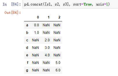
In this case, there is no overlap in the other axis. You can see the sorted index aggregate ('outer'join). You can also pass in join='inner ':
s4 = pd.concat([s1, s3])
s4
#
a    0
b    1
f    5
g    6
dtype: int64
pd.concat([s1, s4], axis=1, sort=True)
#
      0	1
a	0.0	0
b	1.0	1
f	NaN	5
g	NaN	6
pd.concat([s1, s4], axis=1, join='inner', sort=True)
#
    0	1
a	0	0
b	1	1
In this case, the labels for 'f' and 'g' are missing due to the option of join='inner '.
You can even use join axes to specify the axis used to connect other axes:
pd.concat([s1, s4], axis=1, join_axes=[['a', 'c', 'b', 'e']])
#
       0  1
a	0.0	0.0
c	NaN	NaN
b	1.0	1.0
e	NaN	NaN
It is a potential problem that the parts that are spliced together cannot be distinguished in the results. Suppose you want to create a multi-level index on the connection axis, you can use the keys parameter to achieve: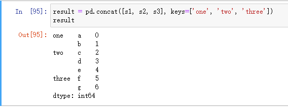
When Series is connected along axis=1, keys become the column header of DataFrame: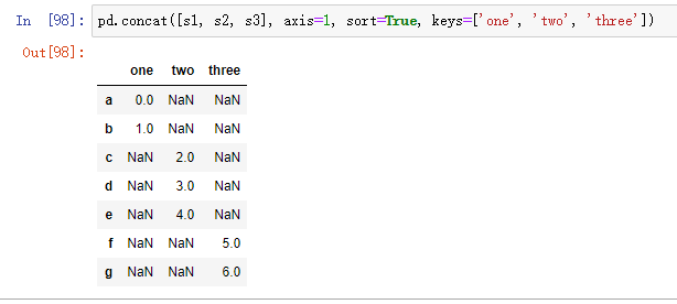
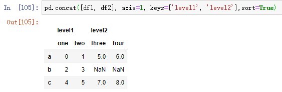
Extend the same logic to the DataFrame object:
df1 = pd.DataFrame(np.arange(6).reshape((3, 2)),index=['a', 'b', 'c'],
                   columns=['one', 'two'])
df2 = pd.DataFrame(5 + np.arange(4).reshape((2, 2)),index=['a', 'c'],
                   columns=['three', 'four'])
df1
#
	one	two
a	  0	  1
b	  2	  3
c	  4	  5
df2
#
  three	four
a	  5	   6
c	  7	   8
If you pass the dictionary of an object instead of a list, the key of the dictionary is used for the keys option: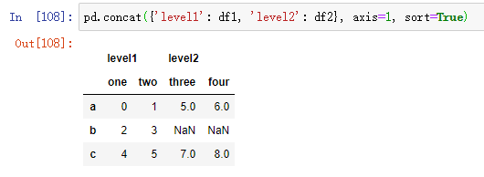
There are also additional parameters responsible for multi-level index generation. For example, we can use the names parameter to name the generated axis level: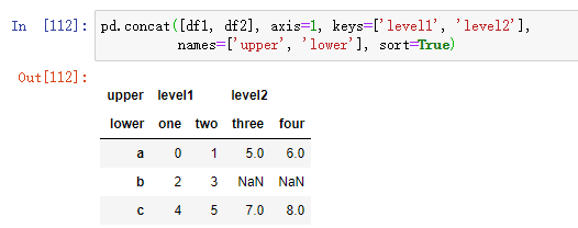
The last thing to consider is the DataFrame that does not contain any related data in the row index: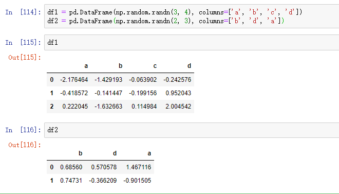
In this example, we pass in ignore_index=True: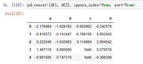
| parameter | describe |
|---|---|
| objs | List or dictionary of pandas objects to connect; this is a required parameter |
| axis | The axis of the connection; default is 0 (along the row direction) |
| join | Can be inner or outer (the default is outer); used to specify whether the connection method is inner or outer |
| join_axes | Specific index used to specify other n-1 axes, which can replace the logic of inner / outer connection |
| keys | The value associated with the object to be connected forms a hierarchical index along the connection axis; it can be a list or array of any value, an array of tuples, or a list of arrays (if multi-level array is passed to the levels parameter) |
| leels | This parameter is used to specify the level of multi-level index when key value is passed |
| names | If a keys and / or levels parameter is passed in, it is used for the hierarchical name of the multi-level index |
| verify_intergrity | Check whether the new axis in the connection object is duplicated, if so, an exception is thrown; the default (False) allows duplicates |
| ingore_index | Instead of keeping the index along the connection axis, a new (total length) index is generated |
2.4 joint overlapping data
There is another data federation scenario, which is neither a merge operation nor a join operation. You may have two datasets whose indexes overlap in whole or in part. As an example, consider Numpy's where function, which can perform array oriented if else equivalent operations:
a = pd.Series([np.nan, 2.5, 0.0, 3.5, 4.5, np.nan],
              index=['f', 'e', 'd', 'c', 'b', 'a'])
b = pd.Series([0, np.nan, 2, np.nan, np.nan, 5.],
              index=['a', 'b', 'c', 'd', 'e', 'f'])
a
#
f    NaN
e    2.5
d    0.0
c    3.5
b    4.5
a    NaN
dtype: float64
b
#
a    0.0
b    NaN
c    2.0
d    NaN
e    NaN
f    5.0
dtype: float64
np.where(pd.isnull(a), b, a)
#
array([0. , 2.5, 0. , 3.5, 4.5, 5. ])
Series has a combine first method, which can be equivalent to the following axial operations using pandas common data alignment logic:
b.combine_first(a)
#
a    0.0
b    4.5
c    2.0
d    0.0
e    2.5
f    5.0
dtype: float64
We can find that the above code is to pass the data in a into b. if the data in b's row is missing, the data in a will be used. If it already exists, the original data is retained.
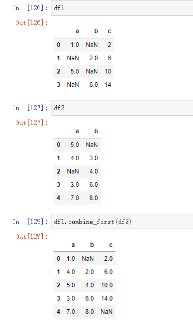
In DataFrame, combine first does the same operation column by column, so you can think that it "fixes" the missing value of the calling object according to the object you passed in:
df1 = pd.DataFrame({'a': [1., np.nan, 5., np.nan],
                    'b': [np.nan, 2., np.nan, 6.],
                    'c': range(2, 18, 4)})
df2 = pd.DataFrame({'a': [5., 4., np.nan, 3., 7.],
                    'b': [np.nan, 3., 4., 6., 8.],})
8.3 remodeling and Perspective
There are several basic operations for rearranging table type data. These operations are called reshaping or perspective.
3.1 reshaping with multi-level index
Multi level indexes provide a consistent way to rearrange data in DataFrame. Here are two basic operations:
stack this operation "rotates" or pivots the data in the column to the row
unstack this operation will pivot the data in the row to the column
Consider a small DataFrame with an array of strings as row and column indexes: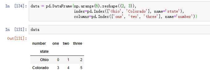
Using the stack method on this data will pivot the column to the row and generate a new Series: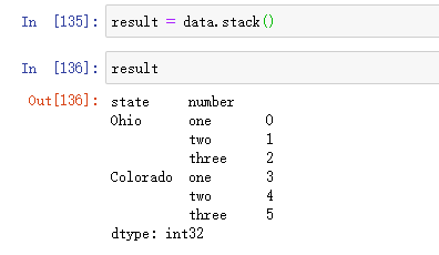
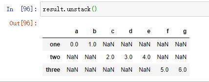
From a multi-level index sequence, you can use the unstack method to rearrange the data into a DataFrame: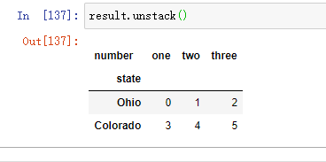
By default, the innermost layer is destacked (as with the unstack method). You can split a different level by passing in a level serial number or name: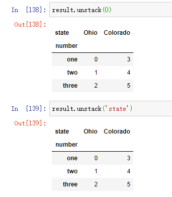
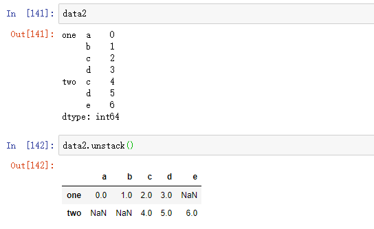
If all values in the hierarchy are not included in each subgroup, splitting may introduce missing values:
s1 = pd.Series([0, 1, 2, 3], index=['a', 'b', 'c', 'd'])
s2 = pd.Series([4, 5, 6], index=['c', 'd', 'e'])
data2 = pd.concat([s1, s2], keys=['one', 'two'])
By default, the stack filters out missing values, so the stack destacking operation is reversible: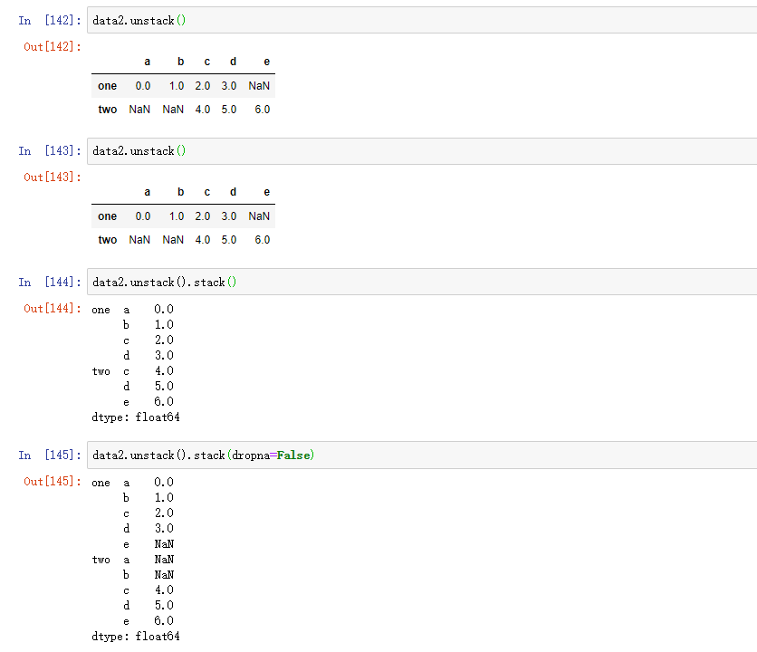
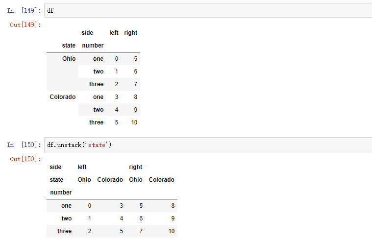
When you destack in DataFrame, the destacked level becomes the lowest level in the result:
df = pd.DataFrame({'left': result, 'right': result + 5},
                  columns=pd.Index(['left', 'right'], name='side'))
When calling the stack method, we can indicate the axial name to stack: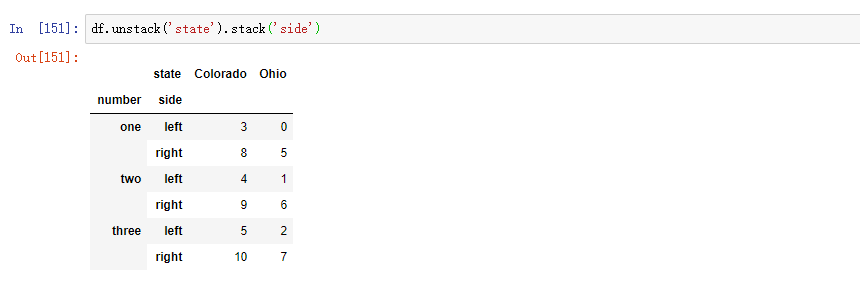
3.2 perspective "long" to "wide"
The way to store multiple time series in database and CSV is called long format or stack format. Let's load some instance data, and then do a few time series regularization and other data cleaning operations:
data = pd.read_csv('macrodata.csv')
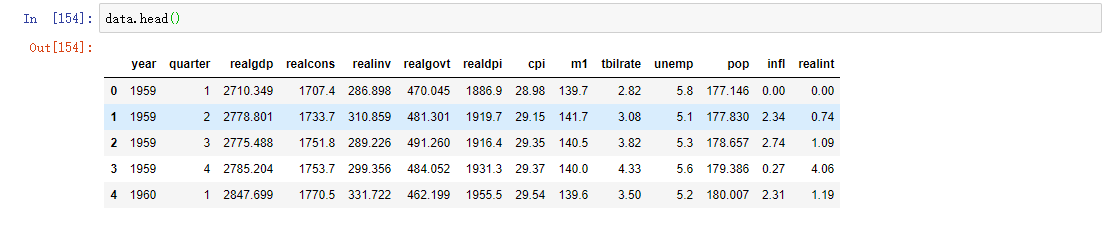
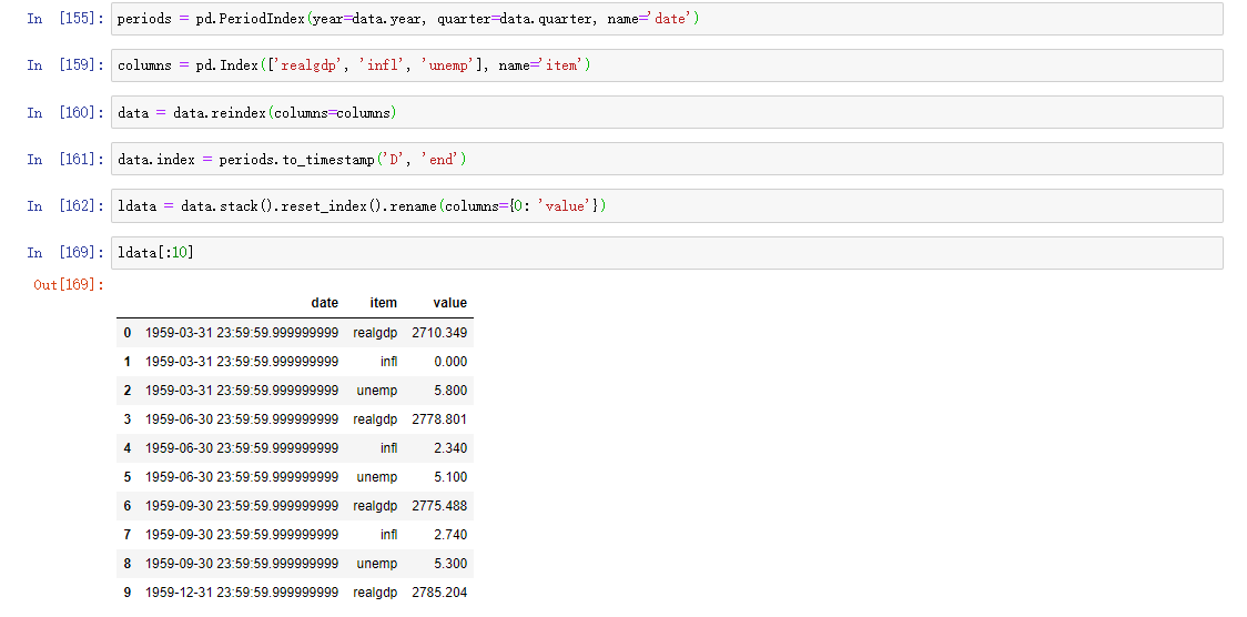
We'll go deeper into PeriodIndex later. Simply put, PeriodIndex combines columns such as year and quarter and generates a time interval type. This kind of data is called long format of multi time series, or other observation data with two or more keys (here, our keys are data and item). Each row in the table represents a single observation at a point in time.
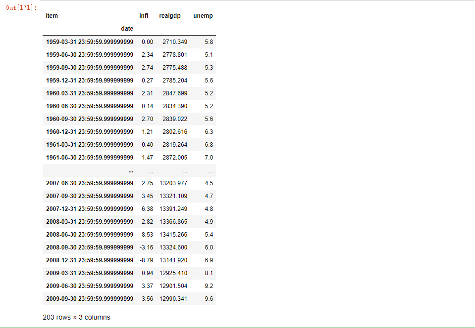
Data is usually stored in a relational database like MySQL in this way, because the fixed pattern (column name and data type) allows the number of different values in the item column to change as the data is added to the table. In the previous example, data and item are usually primary keys (in the case of relational databases), providing relational integrity and simpler connections. In some cases, it's more difficult to deal with data in this format, and you may prefer to get a DataFrame with a separate column for each different item indexed by the date column timestamp. This is the pivot method of DataFrame.
pivoted = ldata.pivot('date', 'item', 'value')
pivoted
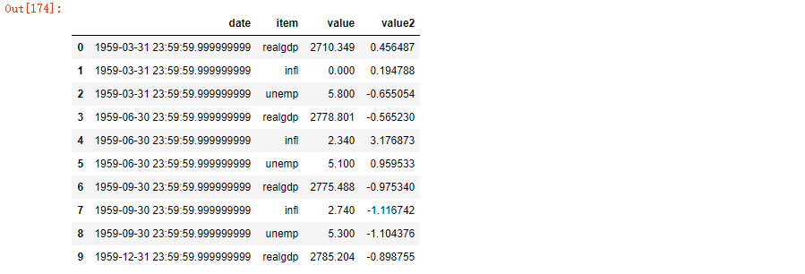
The first two values passed are used as columns for row and column indexes, respectively, followed by optional numeric columns to populate the DataFrame. If you have two series values, you want to reshape them at the same time:
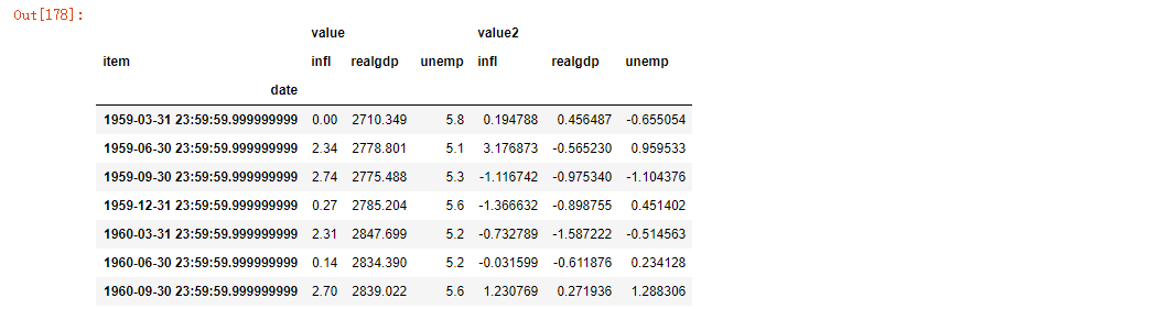
ldata['value2'] = np.random.randn(len(ldata))
ldata[:10]
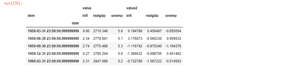
If you omit the last parameter, you will get a DataFrame with multiple columns:
pivoted = ldata.pivot('date', 'item')
pivoted[:5]
pivoted['value'][:5]

Note that the pivot method is equivalent to creating a hierarchical index using set_index, and then calling unstack:
unstacked = ldata.set_index(['date', 'item']).unstack('item')
unstacked[:7]
3.3 perspective "width" into "length"
In DataFrame, the reverse operation of pivot method is pandas.melt. Unlike transforming a column into multiple columns in a new DataFrame, it merges multiple columns into a single column, resulting in a new DataFrame that is longer than the input. Example:
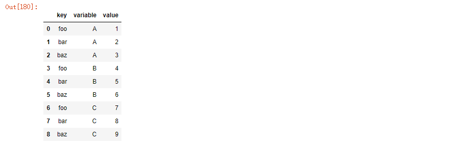
df = pd.DataFrame({'key': ['foo', 'bar', 'baz'],
                   'A': [1, 2, 3],
                   'B': [4, 5, 6],
                   'C': [7, 8, 9]})
df
#
	key	A	B	C
0	foo	1	4	7
1	bar	2	5	8
2	baz	3	6	9
The 'key' column can be used as a grouping label, and other columns are data values. When using panda.melt, we must indicate which columns are grouped indicators, if any. Here, let's use 'key' as the only group indicator:
melted = pd.melt(df, ['key'])
melted
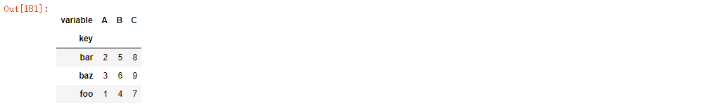
With pivot, we can reshape the data back to its original layout:
reshaped = melted.pivot('key', 'variable', 'value')
reshaped
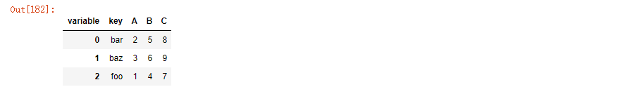
Since the result of pivot generates an index based on the column as the row label, we may want to use reset index to move the data back to a column:
reshaped.reset_index()
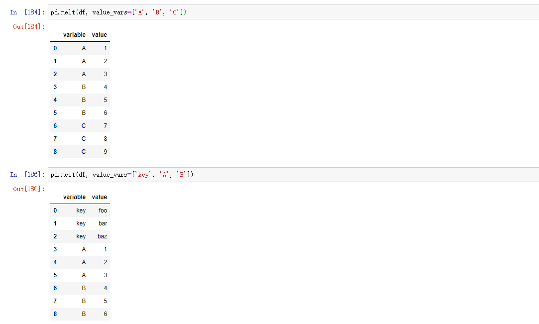
You can also specify a subset of columns as column values:
pd.melt(df, id_vars=['key'], value_vars=['A', 'B'])
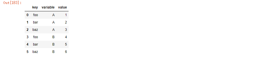
pandas.melt can also be used without any grouping indicators: