Principal Component Analysis and Factor Analysis

#Packet loading
library(corrplot)
library(psych)
library(GPArotation)
library(nFactors)
library(gplots)
library(RColorBrewer)

• 1
• 2
• 3
• 4
• 5
• 6
• 7

principal component analysis

Principal Component Analysis (PCA) is to extract a small number of irrelevant variables for a large number of related variables, these irrelevant variables also become principal component variables.

Data exploration

#In this section, the questionnaire data set of consumer brand perception is introduced as data.

pca <- read.csv("http://r-marketing.r-forge.r-project.org/data/rintro-chapter8.csv")

summary(pca)
#As you can see, except for one character variable, the data are all numeric variables ranging from 1 to 10.
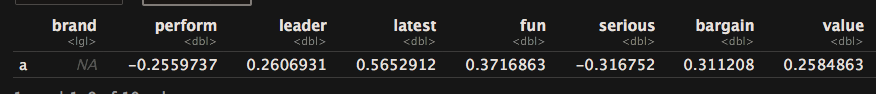
head(pca)

• 1
• 2
• 3
• 4
• 5
• 6
• 7
• 8

library(corrplot)
#Check the correlation between two variables
corrplot(cor(pca[,1:9]), order = "FPC")
#"FPC" for the first principal component order.

• 1
• 2
• 3
• 4
• 5

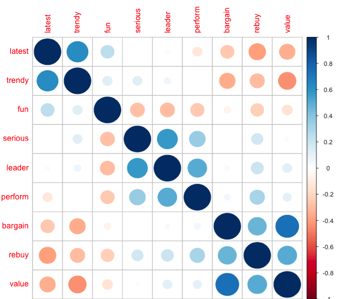
It can be roughly found that they are clustered into three categories: latest/trendy/fun, serious/leader/perform, bargain/rebuy/value, which is also the next analysis to verify.

Extraction of Principal Components

#Data scaling
pca.sc <- pca
pca.sc[,1:9] <- scale(pca.sc[,1:9])
#Extraction of Principal Components
pca.pc <- prcomp(pca.sc[,1:9])
summary(pca.pc)
#Judging the number of components
plot(pca.pc, type = "l")

• 1
• 2
• 3
• 4
• 5
• 6
• 7
• 8

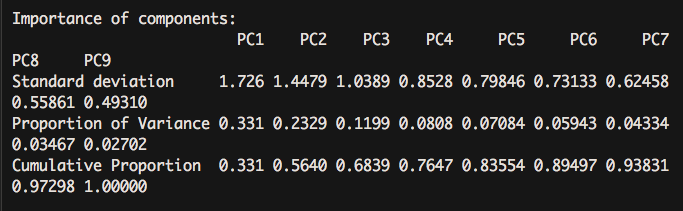
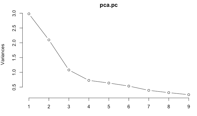
For the number of principal components, scree diagram shows that after three categories, the variance value added of each principal component interpretation decreases.

Principal Component Score Acquisition

#Psh packages also have good PCA analysis output
library(psych)
fa.parallel(pca.sc[,1:9],fa = "pc") #principal() needs to know in advance about the composition of the package and output the lithotripsy map.
pca.psy <- principal(pca.sc[,1:9], nfactors = 3,rotate = "none")
round(unclass(pca.psy$weights),2) #Obtain principal component score

• 1
• 2
• 3
• 4
• 5

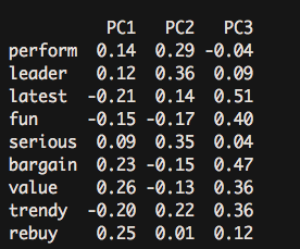
The composition coefficients of each principal component obtained here can be derived as follows: PC1 = 0.14*perform + 0.12 leader + latest(-0.21)... .

Brand Perception Map

At the same time, another important aspect of the application of principal component analysis is to visualize the relationship between different categories (brands) through biplot.

#The first two components of the principal component are mapped to two dimensions, but the direct projection data subject will face the problem of too many scatters and poor visibility.
biplot(pca.pc)
#Therefore, its category (brand) can be mapped.
pca.mean <- aggregate(.~ brand, pca.sc, mean)
rownames(pca.mean) <- pca.mean[,1]
pca.mean.pc <- prcomp(pca.mean[,-1], scale = T)
summary(pca.mean.pc)
biplot(pca.mean.pc) #Brand Perception Map

• 1
• 2
• 3
• 4
• 5
• 6
• 7
• 8
• 9

From this map, we can examine the harmony and position of each category (brand).

The differences among different brands can be further examined.

pca.mean["a",] - pca.mean["j",]

• 1
• 2

Explanatory Factor Analysis

Factor analysis (EFA) is a method used to discover the potential structure of a group of variables. It mainly extracts and obtains observable explicit variables for unobservable factor variables.

DETERMINATION OF EFA FACTOR QUANTITY

# Number of determinants for gravel maps and eigenvalues
library(nFactors)
# Various schemes of gravel maps
nScree(pca.sc[,1:9])

#  noc naf nparallel nkaiser
#  1   3   2         3       3

# Number of eigenvalues > 1
eigen(cor(pca.sc[,1:9]))

#$values
#[1] 2.9792956 2.0965517 1.0792549 0.7272110 0.6375459 0.5348432 0.3901044
#[8] 0.3120464 0.2431469

• 1
• 2
• 3
• 4
• 5
• 6
• 7
• 8
• 9
• 10
• 11
• 12
• 13
• 14
• 15

From the above results, we can see that the factor number is between 2 and 3.

#Extraction of Common Factor by Psh Packet
#Scheme with Common Factor Quantity 2
fa(pca.sc[,1:9], nfactors = 2, rotate = "none",fm = "ml") #Factorization Method Selection of Maximum Likelihood Method ml

• 1
• 2
• 3

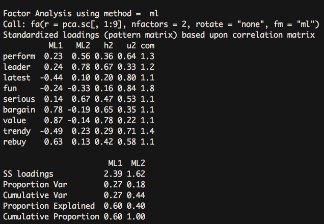
The two-factor scheme explained only 44% of the variance.

#A Scheme with Common Factor Number 3
fa(pca.sc[,1:9], nfactors = 3, rotate = "none",fm = "ml") 

• 1
• 2

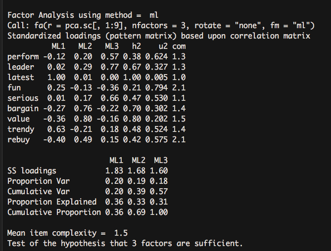
It rose to 57% variance interpretation. It can be concluded that the three-factor scheme is better than the other one.

EFA rotation

Two methods of rotation

#Orthogonal rotation using psych's fa
#Orthogonal rotation
fa.vaf <- fa(pca.sc[,1:9], nfactors = 3, rotate = "varimax",fm = "ml")  
fa.vaf
#Skew rotation
#With oblimin oblique rotation of GPArotation, the result of factanal is relatively concise.
library(GPArotation)
fa.ob <- factanal(pca.sc[,1:9], factors = 3, rotation = "oblimin") 
fa.ob
#Unlisted factor structure matrix is obtained by factor model matrix*factor correlation matrix.
fsm <- function(oblique) {
if (class(oblique)[2]=="fa" & is.null(oblique$rotmat)) {
    warning("Object doesn't look like oblique EFA")
} else {
    P <- unclass(oblique$loading)
    F <- P %*% oblique$rotmat
    return(F)
} }
fsm(fa.ob)

• 1
• 2
• 3
• 4
• 5
• 6
• 7
• 8
• 9
• 10
• 11
• 12
• 13
• 14
• 15
• 16
• 17
• 18
• 19
• 20

Orthogonal rotation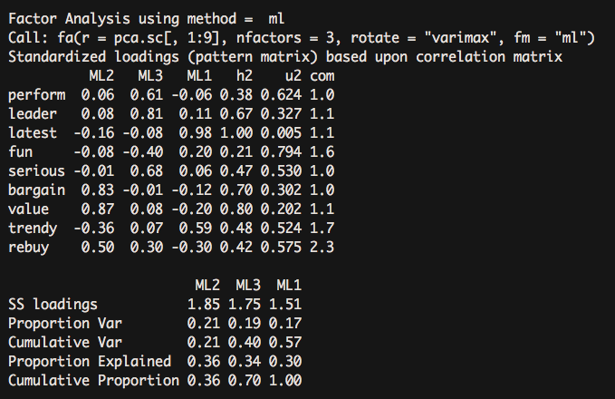

Skew rotation

Orthogonal rotation does not correlate mandatory factors and focuses on the correlation of the variables with the factors. Oblique rotation focuses on three matrices:
* The normalized regression coefficients of each variable and factor variable are listed in the pattern matrix.
* Factor correlation matrix, the correlation between factors.
* Factor structure matrix, i.e. factor load matrix, measures the correlation coefficient between variables and factors.

#Corresponding alternatives
#Orthogonal rotation
fa.va <- factanal(pca.sc[,1:9], factors = 3, rotation = "varimax") 
#Skew rotation
fa.promax <- fa(pca.sc[,1:9], nfactors = 3, rotate = "promax",fm = "ml") 

fsmfa <- function(oblique) {
if (class(oblique)[2]=="fa" & is.null(oblique$Phi)) {
    warning("Object doesn't look like oblique EFA")
} else {
    P <- unclass(oblique$loading)
    F <- P %*% oblique$Phi
    return(F)
} }

fsmfa(fa.promax)

• 1
• 2
• 3
• 4
• 5
• 6
• 7
• 8
• 9
• 10
• 11
• 12
• 13
• 14
• 15
• 16

Visualization of EFA Rotation Results

Roadmap is used to show the relationship between potential factors and individual factors.

fa.diagram(fa.promax,simple = T,digits = 2)

• 1

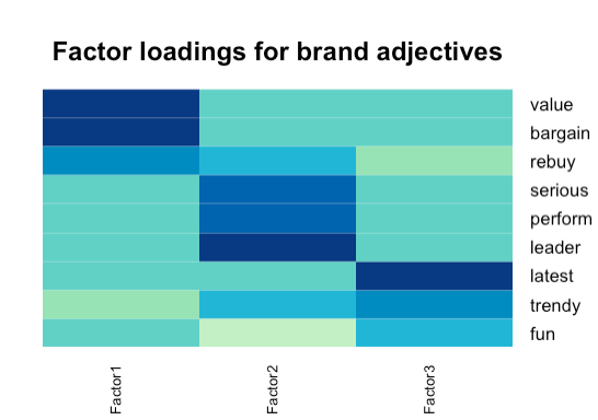
Thermal maps are used to show the relationship between potential factors and variables more intuitively.

library(gplots)
library(RColorBrewer)
heatmap.2(fa.ob$loadings,
          col=brewer.pal(9, "GnBu"), trace="none", key=FALSE, dend="none",
           Colv=FALSE, cexCol = 1.5,
           main="\n\n\nFactor loadings for brand adjectives")

• 1
• 2
• 3
• 4
• 5
• 6

Scores of different brand factors

#Achieving the Mean Value of Three Factors for Each Brand
fa.ob <- factanal(pca.sc[,1:9], factors = 3, rotation = "oblimin",scores = "Bartlett") 
fa.score <- data.frame(fa.ob$scores)
fa.score$brand <- pca.sc$brand
fa.score.mean <- aggregate(.~ brand, fa.score, mean)
fa.score.mean
#Making Thermal Map Based on the Mean Value of Factor
rownames(fa.score.mean) <- fa.score.mean[, 1]           # brand names
fa.score.mean <- fa.score.mean[, -1]

heatmap.2(as.matrix(fa.score.mean),
           col=brewer.pal(9, "GnBu"), trace="none", key=FALSE, dend="none",
           cexCol=1.2, main="\n\n\n\nMean factor score by brand")

• 1
• 2
• 3
• 4
• 5
• 6
• 7
• 8
• 9
• 10
• 11
• 12
• 13
• 14