• List item
  Regression analysis is the core of statistics, usually using one or more predictive variables to predict response variables.
  Regression analysis usually chooses the variables related to response variables as explanatory variables to describe the relationship between them. You can also generate an equation that interprets the response variable with the explanatory variable.
  The lm() function is encapsulated in R to realize single variable and multi variable regression.
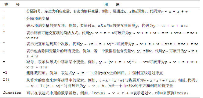
  The symbols in R are described as follows:
  

data(women)
fit<-lm(women$height~women$weight,data=women)
 summary(fit)

Call:
lm(formula = women$height ~ women$weight, data = women)

Residuals:
     Min       1Q   Median       3Q      Max 
-0.83233 -0.26249  0.08314  0.34353  0.49790 

Coefficients:
              Estimate Std. Error t value Pr(>|t|)    
(Intercept)  25.723456   1.043746   24.64 2.68e-12 ***
women$weight  0.287249   0.007588   37.85 1.09e-14 ***
---
Signif. codes:  0 '***' 0.001 '**' 0.01 '*' 0.05 '.' 0.1 ' ' 1

Residual standard error: 0.44 on 13 degrees of freedom
Multiple R-squared:  0.991,	Adjusted R-squared:  0.9903 
F-statistic:  1433 on 1 and 13 DF,  p-value: 1.091e-14
fitted(fit)
       1        2        3        4        5        6 
58.75712 59.33162 60.19336 61.05511 61.91686 62.77861 
       7        8        9       10       11       12 
63.64035 64.50210 65.65110 66.51285 67.66184 68.81084 
      13       14       15 
69.95984 71.39608 72.83233 
residuals(fit)
          1           2           3           4           5 
-0.75711680 -0.33161526 -0.19336294 -0.05511062  0.08314170 
          6           7           8           9          10 
 0.22139402  0.35964634  0.49789866  0.34890175  0.48715407 
         11          12          13          14          15 
 0.33815716  0.18916026  0.04016335 -0.39608278 -0.83232892 

polynomial regression
A quadratic term sq (X) can be added to improve the prediction accuracy of regression

fit<-lm(women$weight~women$height+I(women$height^2),data=women)
summary(fit)

Call:
lm(formula = women$weight ~ women$height + I(women$height^2), 
    data = women)

Residuals:
     Min       1Q   Median       3Q      Max 
-0.50941 -0.29611 -0.00941  0.28615  0.59706 

Coefficients:
                   Estimate Std. Error t value Pr(>|t|)    
(Intercept)       261.87818   25.19677  10.393 2.36e-07 ***
women$height       -7.34832    0.77769  -9.449 6.58e-07 ***
I(women$height^2)   0.08306    0.00598  13.891 9.32e-09 ***
---
Signif. codes:  0 '***' 0.001 '**' 0.01 '*' 0.05 '.' 0.1 ' ' 1

Residual standard error: 0.3841 on 12 degrees of freedom
Multiple R-squared:  0.9995,	Adjusted R-squared:  0.9994 
F-statistic: 1.139e+04 on 2 and 12 DF,  p-value: < 2.2e-16

The results of the analysis can be read, the regression coefficients are very significant, the model variance interpretation rate has increased to 99.9%.
We can also visualize:
plot(womenheight,womenheight,womenheight,womenweight)
lines(women$height,fitted(fit))