Data import and preprocessing
The first is to import all packages required for this data mining
import pandas as pd
import matplotlib.pyplot as plt
import numpy as np
from sklearn.preprocessing import StandardScaler
from sklearn.preprocessing import MinMaxScaler
from sklearn.model_selection import train_test_split
from sklearn.decomposition import PCA
from mpl_toolkits.mplot3d import Axes3D
from sklearn.discriminant_analysis import LinearDiscriminantAnalysis
from sklearn.model_selection import cross_val_score
from sklearn.ensemble import RandomForestClassifier
from sklearn.tree import DecisionTreeClassifier
from sklearn.ensemble import ExtraTreesClassifier
from sklearn.neighbors import KNeighborsClassifier,KNeighborsRegressor
from sklearn.preprocessing import StandardScaler
from sklearn import svm
import seaborn as sns
Next, we import disk data and perform basic processing on the data
file_path='data\smart dataset sample.csv'
df=pd.read_csv(file_path)
data=df.iloc[:,3:]
X=data.iloc[:,1:]
Y=data.iloc[:,0]

# Delete samples with empty features
X.dropna(how='all',inplace=True)
Y=Y.iloc[X.index]

X=X.reset_index(drop=True)
Y=Y.reset_index(drop=True)
The data table df imported at the beginning is shown in the following figure
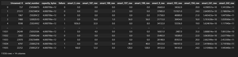
There are 14 fields and 11036 samples. We first remove the first three useless fields to get a new data table data, and then separate the smart feature and label failure into X and Y
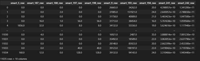
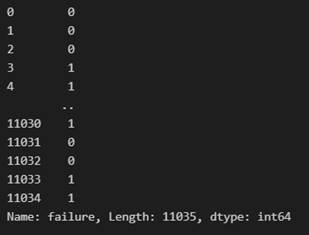
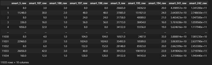
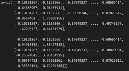
For X, we first delete the disk samples with all empty eigenvalues, delete one sample in total, then synchronously update the data sets X and y, and finally reset the index es of X and Y. the obtained X and y are shown in the figure below
X dataset
Y dataset
Missing value filling
We have a variety of missing value filling methods (mean filling, mode filling, regression filling, self coding neural network filling)
What surprises me is that the data set filled with mean is in cross_ val_ In the score evaluation, the performance is the best. I will analyze this later
KNN_classifier filling
# KNN regression filling vacancy value
from sklearn.neighbors import KNeighborsClassifier,KNeighborsRegressor

def knn_missing_filled(train_x,train_y,test,k=3,dispersed=True):
    if dispersed:
        clf=KNeighborsClassifier(n_neighbors=k,weights='distance',n_jobs=-1)
    else:
        clf=KNeighborsRegressor(n_neighbors=k,weights='distance',n_jobs=-1)
    clf.fit(train_x,train_y)
    return test.index,clf.predict(test)
RandomForest
# randomforest fill gap value

from sklearn.ensemble import RandomForestRegressor,RandomForestClassifier  # Random forest regression

def randomforest_missing_filled(train_x,train_y,test,dispersed=True):
    if dispersed:
        clf=RandomForestClassifier(n_estimators=10)
    else:
        clf=RandomForestRegressor(n_estimators=10)
    clf.fit(train_x,train_y)
    return test.index,clf.predict(test)
Self coding neural network
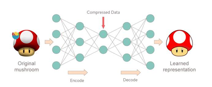
The model example of self coding neural network is shown in the figure above. It encode s and compresses the input, extracts important features, then decode s and restores the data. In essence, it learns a function f W , b ( X ) = X f_{W,b} (X)=X fW,b(X)=X.
We can use the complete data as the training set X X The X-input self coding neural network is used for learning, and the distribution and characteristics of the data are extracted through continuous iteration, and then we will extract the data blocks with missing values X ′ X' The missing value of X 'is filled with random numbers, and then X ′ X' X 'is input into the network for multiple iterations, and the data set is gradually transformed by using the distribution characteristics of the data in the complete data set extracted in the network and other important features extracted X ′ X' X 'restore to fill the data
import random
import pandas as pd
import numpy as np
import matplotlib.pylab as plt
import seaborn as sns
from keras.utils import np_utils
from sklearn.preprocessing import LabelEncoder
from keras.objectives import mse
from keras.models import Sequential
from keras.layers.core import Dropout, Dense
from keras.regularizers import l1_l2
from collections import defaultdict
%matplotlib inline
def make_reconstruction_loss(n_features):
    '''Reconstruction error'''
    def reconstruction_loss(input_and_mask, y_pred):
        X_values = input_and_mask[:, :n_features]
        X_values.name = "$X_values"
        missing_mask = input_and_mask[:, n_features:]
        missing_mask.name = "$missing_mask"
        observed_mask = 1 - missing_mask
        observed_mask.name = "$observed_mask"
        X_values_observed = X_values * observed_mask
        X_values_observed.name = "$X_values_observed"
        pred_observed = y_pred * observed_mask
        pred_observed.name = "$y_pred_observed"
        return mse(y_true=X_values_observed, y_pred=pred_observed)
    return reconstruction_loss
def masked_mae(X_true, X_pred, mask):
    masked_diff = X_true[mask] - X_pred[mask]
    return np.mean(np.abs(masked_diff))
class Autoencoder:
    def __init__(self, data,
                 recurrent_weight=0.5,
                 optimizer="adam",
                 dropout_probability=0.5,
                 hidden_activation="relu",
                 output_activation="sigmoid",
                 init="glorot_normal",
                 l1_penalty=0,
                 l2_penalty=0):
        self.data = data.copy()
        self.recurrent_weight = recurrent_weight
        self.optimizer = optimizer
        self.dropout_probability = dropout_probability
        self.hidden_activation = hidden_activation
        self.output_activation = output_activation
        self.init = init
        self.l1_penalty = l1_penalty
        self.l2_penalty = l2_penalty
    def _get_hidden_layer_sizes(self):
        n_dims = self.data.shape[1]
        return [
            min(2000, 8 * n_dims),
            min(500, 2 * n_dims),
            int(np.ceil(0.5 * n_dims)),
        ]
    def _create_model(self):
        hidden_layer_sizes = self._get_hidden_layer_sizes()
        first_layer_size = hidden_layer_sizes[0]
        n_dims = self.data.shape[1]
        model = Sequential()
        model.add(Dense(
            first_layer_size,
            input_dim= 2 * n_dims,
            activation=self.hidden_activation,
            W_regularizer=l1_l2(self.l1_penalty, self.l2_penalty),
            init=self.init))
        model.add(Dropout(self.dropout_probability))
        for layer_size in hidden_layer_sizes[1:]:
            model.add(Dense(
                layer_size,
                activation=self.hidden_activation,
                W_regularizer=l1_l2(self.l1_penalty, self.l2_penalty),
                init=self.init))
            model.add(Dropout(self.dropout_probability))
        model.add(Dense(
            n_dims,
            activation=self.output_activation,
            W_regularizer=l1_l2(self.l1_penalty, self.l2_penalty),
            init=self.init))
        loss_function = make_reconstruction_loss(n_dims)
        model.compile(optimizer=self.optimizer, loss=loss_function)
        return model
    def fill(self, missing_mask):
        self.data[missing_mask] = -1
    def _create_missing_mask(self):
        if self.data.dtype != "f" and self.data.dtype != "d":
            self.data = self.data.astype(float)
        return np.isnan(self.data)
    def _train_epoch(self, model, missing_mask, batch_size):
        input_with_mask = np.hstack([self.data, missing_mask])
        n_samples = len(input_with_mask)
        n_batches = int(np.ceil(n_samples / batch_size))
        indices = np.arange(n_samples)
        np.random.shuffle(indices)
        X_shuffled = input_with_mask[indices]
        for batch_idx in range(n_batches):
            batch_start = batch_idx * batch_size
            batch_end = (batch_idx + 1) * batch_size
            batch_data = X_shuffled[batch_start:batch_end, :]
            model.train_on_batch(batch_data, batch_data)
        return model.predict(input_with_mask)
    def train(self, batch_size=256, train_epochs=100):
        missing_mask = self._create_missing_mask()
        self.fill(missing_mask)
        self.model = self._create_model()
        observed_mask = ~missing_mask
        for epoch in range(train_epochs):
            X_pred = self._train_epoch(self.model, missing_mask, batch_size)
            observed_mae = masked_mae(X_true=self.data,
                                    X_pred=X_pred,
                                    mask=observed_mask)
            if epoch % 50 == 0:
                print("observed mae:", observed_mae)
            old_weight = (1.0 - self.recurrent_weight)
            self.data[missing_mask] *= old_weight
            pred_missing = X_pred[missing_mask]
            self.data[missing_mask] += self.recurrent_weight * pred_missing
        return self.data.copy()
The filling process is to adopt complete features
'smart_5_raw','smart_187_raw','smart_188_raw','smart_197_raw','smart_198_raw'
And the corresponding label failure is used as the training set to train the learner to learn the hypothesis function f ( x ) f(x) f(x) and calculate the value of vacancy value
The specific process is as follows:
-
Feature smart_198_raw as an example, the data table is divided into two data sets according to this column, the feature smart_ 198_ If raw is not empty, it will be the training set, and if raw is empty, it will be the test set to be predicted
-
Finally, any learning model of sklearn library is used to predict and fill, and the completed data set is obtained
-
Other features with missing values are also operated according to the above process
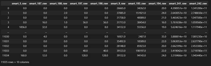
X filled with knn
X filled with mean
Feature distribution visualization
Then, after filling in and obtaining the complete data sets X and Y, we perceptually recognize the data by observing the distribution of features
Visual code
%matplotlib inline
def hist_attribute(df,bin=150):
    '''See how the features are distributed'''
    plt.figure(figsize=[20,25])
    plt.title('feature distribution')
    for i in range(len(df.columns)):
        title=df.columns[i]
        plt.subplot(5,2,i+1)
        plt.hist(df.iloc[:,i].values,bins=bin)
        plt.title(title)
        plt.xlabel('value')
        plt.ylabel('count')
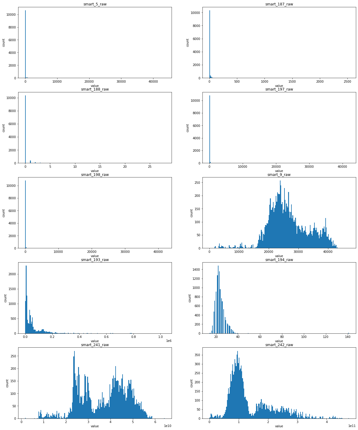
Distribution of features filled with mean / mode
Feature distribution filled by knn/randomForest / self coding neural network
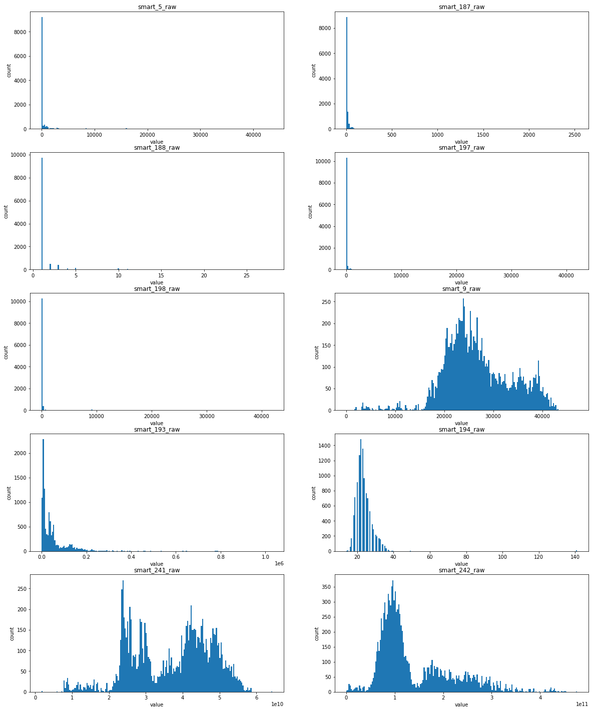
Basically, it can be found that the distribution of the first five features in the figure above is extremely unbalanced, which means that this feature is closely related to whether the hard disk is damaged or not
Explanation: some smart values record the number of abnormal behaviors (restart, high-intensity read-write, etc.) of the hard disk. If these times are small or even 0, it means that the hard disk is working normally. If they are large, it means that the hard disk is damaged
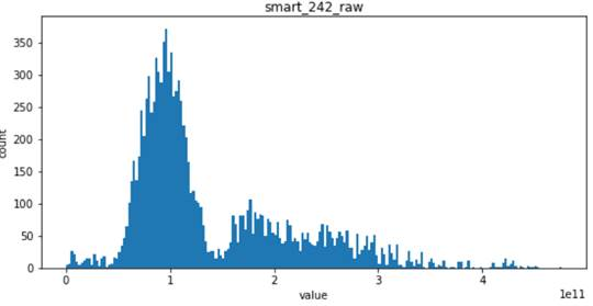
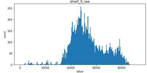
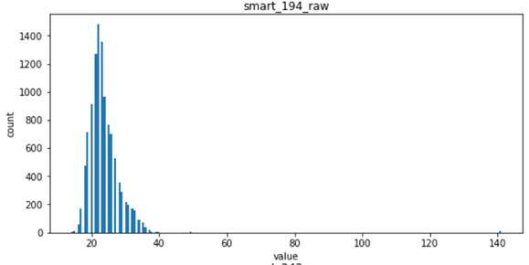
For the latter five features
- For smart_193_raw, which obeys exponential distribution, has a high correlation with sample labels
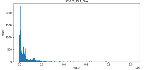
- For the following four features, smart_241_raw, smart_242_raw, smart_9_raw, smart_194_raw, which all obey the single Gaussian distribution or the mixed distribution of the combination of two Gaussian distributions, is the natural feature of the disk sample and has low correlation with the label of the sample (natural random events generally obey the Gaussian distribution)

Viewing correlations between features
%matplotlib inline
complete_features=X
# Draw thermal diagram
plt.figure(figsize=(10,10))
sns.heatmap(complete_features.corr(),annot=True)
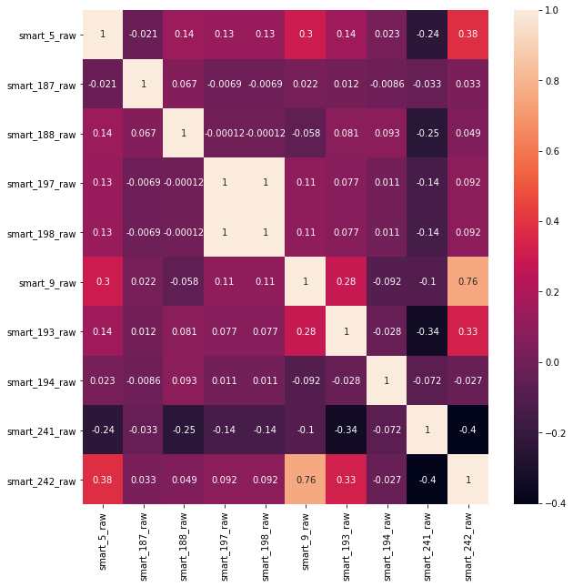
It can be seen that the correlation between the characteristics of the data is not particularly strong and will not have a great impact on the classification task
normalization
# normalization
from sklearn.preprocessing import StandardScaler
from sklearn.preprocessing import MaxAbsScaler

# X=all_log(X)

ss=StandardScaler()
ms=MaxAbsScaler()
X_norm=ss.fit_transform(X)
# X_norm=ms.fit_transform(X)
y_norm=np.array(Y.values).reshape(-1,1)
PCA, dimensionality reduction, sample point distribution, visualization
def plot_pca(num,data,label):
    pca=PCA(n_components=num)
    X_pca=pca.fit_transform(data)
    # Split data
    X_failure=np.array([x for i,x in enumerate(X_pca) if label[i][0]==1])
    X_healthy=np.array([x for i,x in enumerate(X_pca) if label[i][0]==0])

    if num==3:
        fig = plt.figure()
        ax = Axes3D(fig)
        #ax.legend(loc='best')
        ax.set_zlabel('Z', fontdict={'size': 15, 'color': 'red'})
        ax.set_ylabel('Y', fontdict={'size': 15, 'color': 'red'})
        ax.set_xlabel('X', fontdict={'size': 15, 'color': 'red'})
        ax.scatter(X_failure[:,0], X_failure[:,1], X_failure[:,2])
        ax.scatter(X_healthy[:,0], X_healthy[:,1], X_healthy[:,2])
    elif num==2:
        plt.figure(figsize=[10,10])
        plt.scatter(X_failure[:,0],X_failure[:,1])
        plt.scatter(X_healthy[:,0],X_healthy[:,1])
    else:
        print('i do not want to work.....')
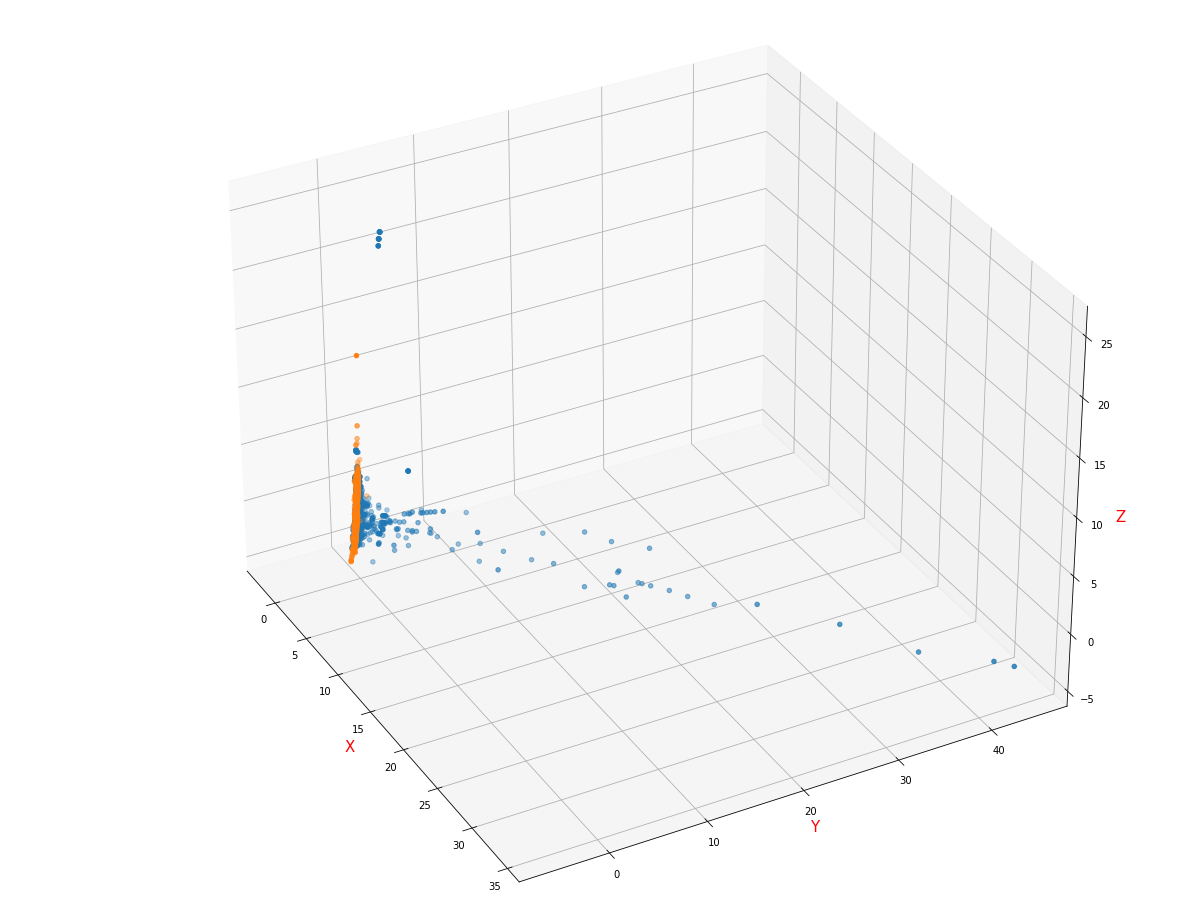
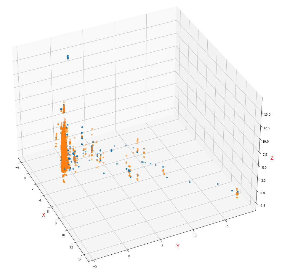
# Dimensionality reduction visualization
%matplotlib auto
plot_pca(num=3,data=X_norm,label=y_norm)
- The visual image of sample distribution is filled with mean / mode, normalized by StandardScaler and reduced to 3D by PCA
It can be found that there is roughly a hyperplane in the three-dimensional feature space, which can be divided
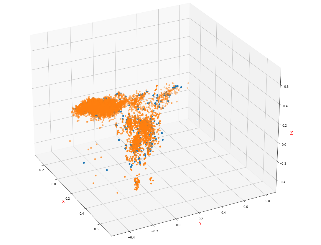
- The visual image of sample distribution is filled with mean / mode, normalized by MaxAbsScaler and reduced to 3D by PCA
It can be seen that the samples are basically not linearly classified (paste into a cluster), and it is speculated that the normalization method destroys the distribution of the data
- KNN/RandomForest / self coding neural network is used to fill the sample distribution visual image, which is normalized by StandardScaler and reduced to 3D by PCA
Compared with the data filled with mean / mode, the dimension with obvious distinction between the distribution of failed samples and health samples is destroyed, which is the direct reason for adopting mean filling
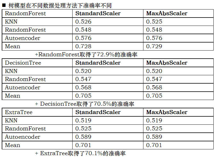
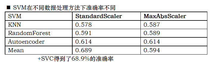
Accuracy test of different learners for data set
In this experiment, five kinds of learners are used to learn the data set
Conclusion:
Accuracy: 8 hidden layer fully connected neural network > (randomforest > decisiontree > extratree) > SVM_ classiier
In the following table, the left side is the method used to fill in the missing value, and the above is the method used for normalization
Test code
- Tree model and SVM model
import warnings
warnings.filterwarnings("ignore")
clf_1 = RandomForestClassifier(n_estimators=10, max_depth=None, min_samples_split=2, random_state=0)
clf_2 = DecisionTreeClassifier(max_depth=None, min_samples_split=2,random_state=0)
clf_3 = ExtraTreesClassifier(n_estimators=10, max_depth=None, min_samples_split=2, random_state=0)
# clf_4=svm.SVC()
# clf_4 = svm.SVC(C=1.0, kernel='rbf', degree=3, gamma='auto', coef0=0.0, shrinking=True,
#                 probability=False, tol=0.001, cache_size=200, class_weight=None,
#                 verbose=False, max_iter=-1, decision_function_shape='ovr',
#                 random_state=None)

scores1 = cross_val_score(clf_1, X_norm, y_norm, cv=5)
scores2 = cross_val_score(clf_2, X_norm, y_norm, cv=5)
scores3 = cross_val_score(clf_3, X_norm, y_norm, cv=5)
# scores4 = cross_val_score(clf_4, X_norm, y_norm, cv=5)

print('RandomForestClassifier scores: ',scores1.mean())
print('DecisionTreeClassifier scores: ',scores2.mean())
print('ExtraTreesClassifier scores: ',scores3.mean())
# print('SVC scores: ',scores4.mean())
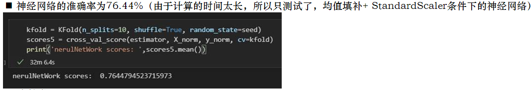
- 8 hidden layer neural network model
# Try neural network classification
from keras.models import Sequential
from keras.layers import Dense
from keras.wrappers.scikit_learn import KerasClassifier
from keras.utils import np_utils
from sklearn.model_selection import KFold
seed = 7
np.random.seed(seed)
# define baseline model
def baseline_model():
    # create model
    model = Sequential()
    model.add(Dense(8, input_dim=10, activation='relu'))
    model.add(Dense(2, activation='softmax'))
    # Compile model
    model.compile(loss='sparse_categorical_crossentropy', optimizer='adam', metrics=['accuracy'])
    return model
estimator = KerasClassifier(build_fn=baseline_model, epochs=200, batch_size=5, verbose=0)
# splitting data into training set and test set. If random_state is set to an integer, the split datasets are fixed.
X_train, X_test, Y_train, Y_test = train_test_split(X_norm, y_norm, test_size=0.3, random_state=0)
estimator.fit(X_train, Y_train)

kfold = KFold(n_splits=10, shuffle=True, random_state=seed)
scores5 = cross_val_score(estimator, X_norm, y_norm, cv=kfold)
print('nerulNetWork scores: ',scores5.mean())
summary
This is the author's first relatively complete data mining experiment. If there are deficiencies, please don't hesitate to give advice!