1. Model construction
1.1 get modeling data
#Read raw data
train = pd.read_csv('train.csv')

#Read cleaned data set
data = pd.read_csv('clear_data.csv')
1.2 select appropriate model
Before model selection, we need to know whether the data set is finally supervised learning or unsupervised learning
Machine learning is mainly divided into two categories
- Supervised learning: teach the computer how to complete the prediction task (with feedback), give a certain amount of data input and corresponding results in advance, that is, training set, modeling and fitting, and finally let the computer predict the results of unknown data.
- Unsupervised learning: compared with supervised learning, there will be no artificially labeled results (no feedback) in the training set. We will not give the results or know what the results of the training set are. Instead, the computer will analyze them by itself through unsupervised learning algorithm, so as to "get the results". Computers may classify a specific data set into several different clusters, so it is called clustering algorithm
The main difference between the two is whether it is necessary to manually participate in the annotation of data results.
On the one hand, the choice of model is determined by our task. In addition to selecting models according to our tasks, we can also decide according to the sample size of data and the sparsity of features. At first, we always try to use a basic model as its baseline, then train other models for comparison, and finally select models with better generalization ability or performance. Here, we use a library (sklearn) most commonly used in machine learning To complete the construction of our model
1.3 cutting training set and test set
# The data set is divided using the set aside method
# The set aside method directly divides the data set into two mutually exclusive sets, one of which is used as the training set and the remaining set as the test set
# The data set is divided into independent variables and dependent variables
# Cut the training set and test set in proportion (the proportion of general test set is 30%, 25%, 20%, 15% and 10%)
# test_size=0.30
# Using stratified sampling
# random_state=0
# Set random seeds so that the results can be reproduced

# Generally, x and y are taken out before cutting. In some cases, uncut ones will be used. At this time, x and y can be used. x is the cleaned data and Y is the survival data we want to predict, 'Survived'
X = data
y = train['Survived']

# The data set is cut and divided according to the proportion of y, and the random seed is 0
X_train, X_test, y_train, y_test = train_test_split(X, y, stratify=y, random_state=0)
# View data shapes
print(X_train.shape, X_test.shape)
Method of dividing training base https://blog.csdn.net/cczx139/article/details/80264492? ops_ request_ misc=&request_ id=&biz_ id=102&utm_ term=%E5%88%92%E5%88%86%E8%AE%AD%E7%BB%83%E9%9B%86%E5%92%8C%E6%B5%8B%E8%AF%95%E9%9B%86&utm_ medium=distribute.pc_ search_ result.none-task-blog-2~all~sobaiduweb~default-3-80264492.pc_ search_ es_ clickV2&spm=1018.2226.3001.4187 https://blog.csdn.net/cczx139/article/details/80264492?ops_request_misc=&request_id=&biz_id=102&utm_term=%E5%88%92%E5%88%86%E8%AE%AD%E7%BB%83%E9%9B%86%E5%92%8C%E6%B5%8B%E8%AF%95%E9%9B%86&utm_medium=distribute.pc_search_result.none-task-blog-2~all~sobaiduweb~default-3-80264492.pc_search_es_clickV2&spm=1018.2226.3001.4187
1.4 model establishment
Steps of model establishment
1. Create a linear model based classification model (logistic regression ()) or a tree based classification model (decision tree, random forest, RandomForestClassifier ())
2. Use these models to train and get the scores of training set and test set respectively
3. View the parameters of the model, change the parameter values, and observe the changes of the model
# RandomForestClassifier() parameter
RandomForestClassifier(bootstrap=True, class_weight=None, criterion='gini', max_depth=None, max_features='auto', max_leaf_nodes=None, min_impurity_decrease=0.0, min_impurity_split=None, min_samples_leaf=1, min_samples_split=2, min_weight_fraction_leaf=0.0, n_estimators=10, n_jobs=None, oob_score=False, random_state=None, verbose=0, warm_start=False)
#LogisticRegression() parameter
LogisticRegression(C=50, class_weight=None, dual=False, fit_intercept=True, intercept_scaling=1, l1_ratio=None, max_iter=100, multi_class='warn', n_jobs=None, penalty='l2', random_state=None, solver='warn', tol=0.0001, verbose=0, warm_start=False)
# Logistic regression is not a regression model, but a classification model, which should not be confused with linear regression
# Random forest is actually decision tree integration in order to reduce the over fitting of decision tree
# The module of linear model is sklearn.linear_model
# The module where the tree model is located is sklearn.ensemble
# Default parameter logistic regression model
# lr = LogisticRegression(max_iter=1000)#Default max_iter=100.
# lr.fit(X_train, y_train)


# Logistic regression model after adjusting parameters
# lr2 = LogisticRegression(C=50,max_iter=1000)#C stands for regularization. The smaller C, the stronger the regularization
# lr2.fit(X_train, y_train)
# Random forest classification model with default parameters
rfc = RandomForestClassifier()
rfc.fit(X_train, y_train)
1.5 output model prediction results
# The general supervision model has a predict in sklearn, which can output the prediction tag_ Proba can output label probability
# Forecast label
pred = lr.predict(X_train)
# At this point, we can see an array of 0 and 1
print(pred[:10])
# Predicted tag probability
pred_proba = lr.predict_proba(X_train)
#
print(pred_proba[:10])
The probability of the prediction label indicates the degree of confidence of the model in the prediction results. With probability, we can calculate the information entropy of the prediction label. The greater the information entropy, the less confidence the model has in the prediction results, which indicates that the input of the model may be too different from the training samples, so it becomes an anomaly detection method.
We can also use the probability of predicted tags for ensemble learning, such as soft voting.
2. Evaluation of the model
#Model evaluation is to know the generalization ability of the model.
#Cross validation is a statistical method to evaluate generalization performance. It is more stable and comprehensive than the method of dividing training set and test set.
#In cross validation, the data is divided many times and multiple models need to be trained.
#The most commonly used cross validation is k-fold cross validation, where k is the number specified by the user, usually 5 or 10.
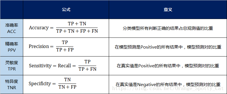
#Accuracy measures how many samples are predicted to be positive examples
#recall measures how many positive samples are predicted to be positive
#f-score is the harmonic average of accuracy and recall
2.1 cross validation
# Task 1: cross validation
# 10 fold cross validation was used to evaluate the previous logistic regression model
# Calculate the average of cross validation accuracy
#Tip: cross validation
# i=Image.open('Snipaste_2020-01-05_16-37-56.png')
# plt.figure("dd")
# plt.imshow(i)
# plt.show()
# Image('Snipaste_2020-01-05_16-37-56.png')

from sklearn.model_selection import cross_val_score
lr = LogisticRegression(C=100,max_iter=1000)
# k-fold cross validation score
scores = cross_val_score(lr, X_train, y_train, cv=10)
print(scores)


# Average cross validation score
print("Average cross-validation score: {:.2f}".format(scores.mean()))\
What impact will the more k-fold bring?
The more K-fold, the more data used as the training set and the less data used as the verification set in a single training verification. The average result will be more reliable, but the total time will also increase. (a large amount of data is exchanged for reliable results, but 2 time increases.)
2.2 confusion matrix
Confusion matrix: also known as possibility table or error matrix. It is a specific matrix used to present the visualization effect of algorithm performance, usually supervised learning (unsupervised learning, usually using matching matrix). Each column represents the predicted value and each row represents the actual category. The name comes from the fact that it can easily indicate whether multiple categories are confused (that is, one class is predicted to be another class).
The value on the diagonal is correct.
# The confusion matrix requires the input of real labels and prediction labels
# Classification can be used for accuracy, recall and f-score_ Report module

# Training model
lr = LogisticRegression(C=10,max_iter=1000)
lr.fit(X_train, y_train)
# Model prediction results
pred = lr.predict(X_train)

# Confusion matrix
confusion_matrix(y_train, pred)

from sklearn.metrics import classification_report

# Accuracy, recall and F1 score
print(classification_report(y_train, pred))
2.3 ROC curve
# The larger the area surrounded by the ROC curve, the better
fpr, tpr, thresholds = roc_curve(y_test, lr.decision_function(X_test))
plt.plot(fpr, tpr, label="ROC Curve")
plt.xlabel("FPR")
plt.ylabel("TPR (recall)")
# The threshold closest to 0 was found
close_zero = np.argmin(np.abs(thresholds))
plt.plot(fpr[close_zero], tpr[close_zero], 'o', markersize=10, label="threshold zero", fillstyle="none", c='k', mew=2)
plt.legend(loc=4)
plt.show()