1, The extended modules for data analysis, scientific computing and visualization are mainly: numpy, scipy, pandas, symphony, matplotlib, Traits, TraitsUI, Chaco, TVTK, Mayavi, VPython, OpenCV.
1.numpy module: scientific computing package, which supports N-dimensional array operation, large matrix processing, mature broadcast function library, vector operation, linear algebra, Fourier transform, random number generation, and can be seamlessly combined with C++ /Fortran language. The default installation of Python v3 already includes numpy.
(1) Import module: import numpy as np
Slice operation
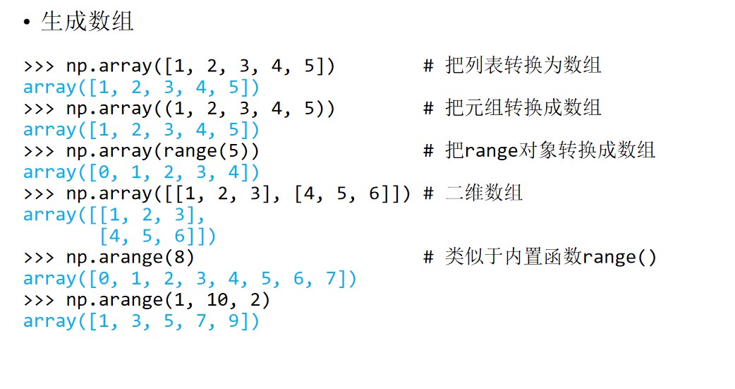
>>> a = np.arange(10)
>>> a
array([0, 1, 2, 3, 4, 5, 6, 7, 8, 9])
>>> a[::-1] # Reverse slice
array([9, 8, 7, 6, 5, 4, 3, 2, 1, 0])
>>> a[::2] # Take one element after another
array([0, 2, 4, 6, 8])
>>> a[:5] # Top 5 elements
array([0, 1, 2, 3, 4])
>>> c = np.arange(25) # Create array
>>> c.shape = 5,5 # Modify array size
>>> c
array([[ 0, 1, 2, 3, 4],
[ 5, 6, 7, 8, 9],
[10, 11, 12, 13, 14],
[15, 16, 17, 18, 19],
[20, 21, 22, 23, 24]])
>>> c[0, 2:5] # Element value between subscripts [2,5] in row 0
array([2, 3, 4])
>>> c[1] # All elements on line 0
array([5, 6, 7, 8, 9])
>>> c[2:5, 2:5] # Element values with row and column subscripts between [2,5]
array([[12, 13, 14],
[17, 18, 19],
[22, 23, 24]])
Boolean operation
>>> x = np.random.rand(10) # An array of 10 random numbers
>>> x
array([ 0.56707504,  0.07527513,  0.0149213 ,  0.49157657,  0.75404095,
      0.40330683,  0.90158037,  0.36465894,  0.37620859,  0.62250594])
>>> x > 0.5               # Compare whether the value of each element in the array is greater than 0.5
array([ True, False, False, False,  True, False,  True, False, False,  True], dtype=bool)
>>> x[x>0.5]              # Gets the elements greater than 0.5 in the array, which can be used to detect and filter exception values
array([ 0.56707504,  0.75404095,  0.90158037,  0.62250594])
>>> x < 0.5
array([False,  True,  True,  True, False,  True, False,  True,  True, False], dtype=bool)
>>> np.all(x<1)           # Test if all elements are less than 1
True
>>> np.any([1,2,3,4])         # Is there an element equivalent to True
True
>>> np.any([0])
False
>>> a = np.array([1, 2, 3])
>>> b = np.array([3, 2, 1])
>>> a > b                     # Comparison of elements in corresponding positions in two arrays
array([False, False,  True], dtype=bool)
>>> a[a>b]
array([3])
>>> a == b
array([False,  True, False], dtype=bool)
>>> a[a==b]
array([2])
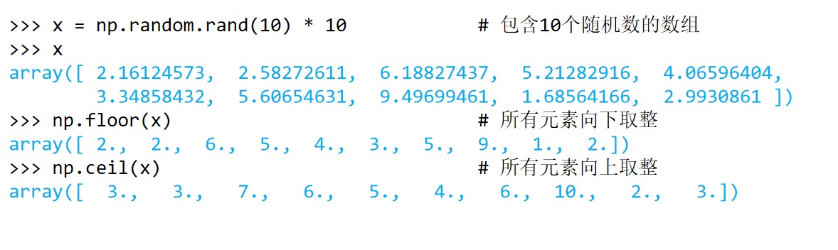
Rounding operation

>>> x = np.random.rand(10)*50      # 10 random numbers
>>> x
array([ 43.85639765,  30.47354735,  43.68965984,  38.92963767,
         9.20056878,  21.34765863,   4.61037809,  17.99941701,
        19.70232038,  30.05059154])
>>> np.int64(x)                    # Rounding
array([43, 30, 43, 38,  9, 21,  4, 17, 19, 30], dtype=int64)
>>> np.int32(x)
array([43, 30, 43, 38,  9, 21,  4, 17, 19, 30])
>>> np.int16(x)
array([43, 30, 43, 38,  9, 21,  4, 17, 19, 30], dtype=int16)
>>> np.int8(x)
array([43, 30, 43, 38,  9, 21,  4, 17, 19, 30], dtype=int8)
Radio broadcast

>>> a = np.arange(0,60,10).reshape(-1,1)     # Column vector
>>> b = np.arange(0,6)                       # Row vector
>>> a
array([[ 0],
       [10],
       [20],
       [30],
       [40],
       [50]])
>>> b
array([0, 1, 2, 3, 4, 5])
>>> a[0] + b                                 # Addition of array and scalar
array([0, 1, 2, 3, 4, 5])
>>> a[1] + b
array([10, 11, 12, 13, 14, 15])
>>> a + b
array([[ 0,  1,  2,  3,  4,  5],
       [10, 11, 12, 13, 14, 15],
       [20, 21, 22, 23, 24, 25],
       [30, 31, 32, 33, 34, 35],
       [40, 41, 42, 43, 44, 45],
       [50, 51, 52, 53, 54, 55]])
>>> a * b
array([[  0,   0,   0,   0,   0,   0],
       [  0,  10,  20,  30,  40,  50],
       [  0,  20,  40,  60,  80, 100],
       [  0,  30,  60,  90,  120, 150],
       [  0,  40,  80,  120, 160, 200],
       [  0,  50,  100, 150,  200, 250]])
Piecewise function
>>> x = np.random.randint(0, 10, size=(1,10))
>>> x
array([[0, 4, 3, 3, 8, 4, 7, 3, 1, 7]])
>>> np.where(x<5, 0, 1) # Element values less than 5 correspond to 0, others correspond to 1
array([[0, 0, 0, 0, 1, 0, 1, 0, 0, 1]])
>>> np.piecewise(x, [x<4, x>7], [lambda x:x*2, lambda x:x*3])
# Elements less than 4 times 2
# Elements greater than 7 times 3
# Other elements change to 0
array([[ 0, 0, 6, 6, 24, 0, 0, 6, 2, 0]])
//Calculate unique value and occurrence times
>>> x = np.random.randint(0, 10, 7)
>>> x
array([8, 7, 7, 5, 3, 8, 0])
>>> np.bincount(x) # Element occurrence, 0 occurrence, 1 occurrence,
# 1. 2 does not appear, 3 appears once, and so on
array([1, 0, 0, 1, 0, 1, 0, 2, 2], dtype=int64)
>>> np.sum(_) # The sum of the occurrence times of all elements is equal to the array length
7
>>> np.unique(x) # Return unique element value
array([0, 3, 5, 7, 8])
//Matrix operation
>>> a_list = [3, 5, 7]
>>> a_mat = np.matrix(a_list) # Create matrix
>>> a_mat
matrix([[3, 5, 7]])
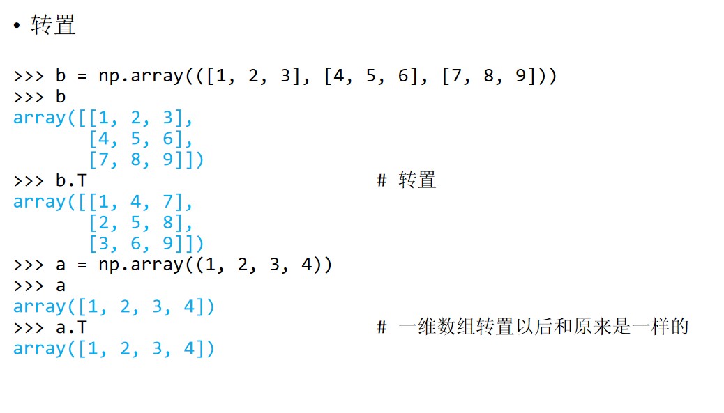
>>> a_mat.T # Matrix transpose
matrix([[3],
[5],
[7]])
>>> a_mat.shape # Matrix shape
(1, 3)
>>> a_mat.size # Number of elements
3
>>> a_mat.mean() # Element average
5.0
>>> a_mat.sum() # Sum of all elements
15
>>> a_mat.max() # Maximum
7
>>> a_mat.max(axis=1) # Transverse maximum
matrix([[7]])
>>> a_mat.max(axis=0) # Longitudinal maximum
matrix([[3, 5, 7]])
>>> b_mat = np.matrix((1, 2, 3)) # Create matrix
>>> b_mat
matrix([[1, 2, 3]])
>>> a_mat * b_mat.T # matrix multiplication
matrix([[34]])
>>> c_mat = np.matrix([[1, 5, 3], [2, 9, 6]]) # Create a 2D matrix
>>> c_mat
matrix([[1, 5, 3],
[2, 9, 6]])
>>> c_mat.argsort(axis=0) # Element sequence number after vertical sorting
matrix([[0, 0, 0],
[1, 1, 1]], dtype=int64)
>>> c_mat.argsort(axis=1) # Element sequence number after horizontal sorting
matrix([[0, 2, 1],
[0, 2, 1]], dtype=int64)
>>> d_mat = np.matrix([[1, 2, 3], [4, 5, 6], [7, 8, 9]])
>>> d_mat.diagonal() # Matrix diagonal element
matrix([[1, 5, 9]])
Calculation on different dimensions of matrix

>>> x = np.matrix(np.arange(0,10).reshape(2,5))  # Two dimensional matrix
>>> x
matrix([[0, 1, 2, 3, 4],
        [5, 6, 7, 8, 9]])
>>> x.sum()                                      # Sum of all elements
45
>>> x.sum(axis=0)                                # Longitudinal summation
matrix([[ 5,  7,  9, 11, 13]])
>>> x.sum(axis=1)                                # Horizontal summation
matrix([[10],
        [35]])
>>> x.mean()                                     # average value
4.5
>>> x.mean(axis=1)
matrix([[ 2.],
        [ 7.]])
>>> x.mean(axis=0)
matrix([[ 2.5,  3.5,  4.5,  5.5,  6.5]])

>>> x.max()                                # Maximum of all elements
9
>>> x.max(axis=0)                          # Longitudinal maximum
matrix([[5, 6, 7, 8, 9]])
>>> x.max(axis=1)                          # Transverse maximum
matrix([[4],
        [9]])
>>> weight = [0.3, 0.7]                    # weight
>>> np.average(x, axis=0, weights=weight)
matrix([[ 3.5,  4.5,  5.5,  6.5,  7.5]])

>>> x = np.matrix(np.random.randint(0, 10, size=(3,3)))
>>> x
matrix([[3, 7, 4],
        [5, 1, 8],
        [2, 7, 0]])
>>> x.std()                         # standard deviation
2.6851213274654606
>>> x.std(axis=1)                   # Transverse standard deviation
matrix([[ 1.69967317],
        [ 2.86744176],
        [ 2.94392029]])
>>> x.std(axis=0)                   # Longitudinal standard deviation
matrix([[ 1.24721913,  2.82842712,  3.26598632]])
>>> x.var(axis=0)                   # Longitudinal variance
matrix([[  1.55555556,   8.        ,  10.66666667]])
2.matplotlib module: depending on numpy module and tkinter module, it can draw many kinds of graphs, including line graph, histogram, pie graph, scatter graph, error line graph, etc. the graph quality can meet the publishing requirements, and it is an important tool for data visualization.
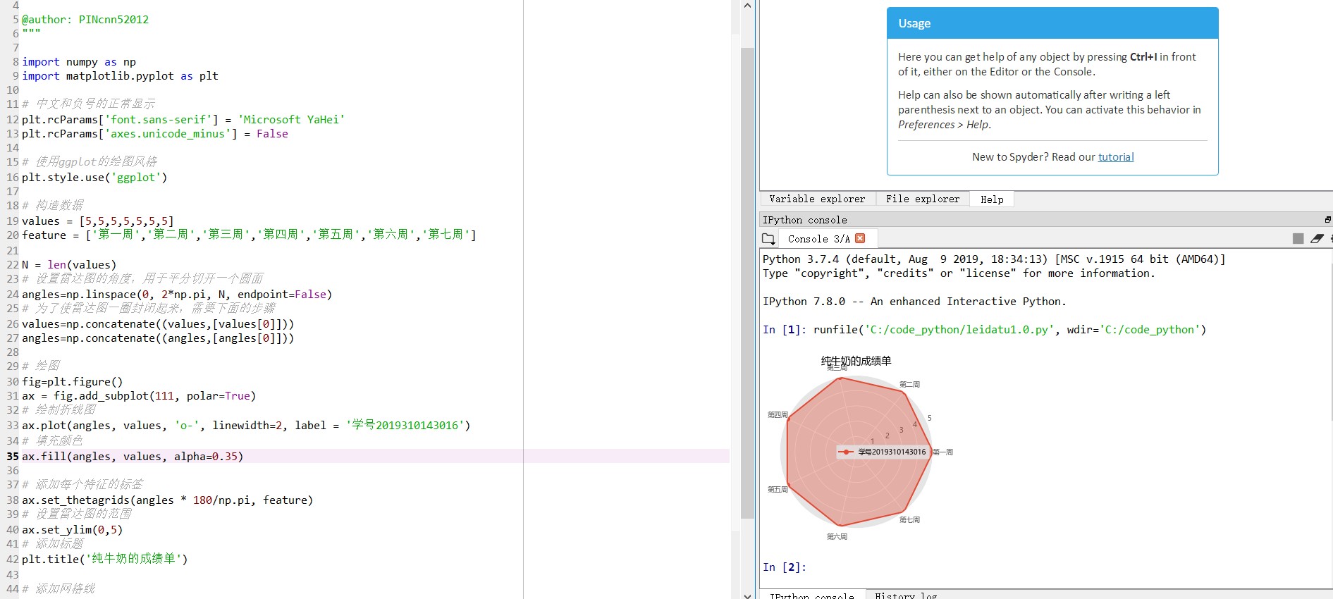
2, Using numpy and matplotlib module to draw radar map
import numpy as np
import matplotlib.pyplot as plt

# Normal display of Chinese and minus sign
plt.rcParams['font.sans-serif'] = 'Microsoft YaHei'
plt.rcParams['axes.unicode_minus'] = False

# Using ggplot's drawing style
plt.style.use('ggplot')

# Construction data
values = [5,5,5,5,5,5,5]
feature = ['Week 1','Week 2','Week 3','Fourth week','Week 5','Week 6','Week 7']

N = len(values)
# Set the angle of the radar chart to bisect a circular surface
angles=np.linspace(0, 2*np.pi, N, endpoint=False)
# In order to close the radar chart, the following steps are required
values=np.concatenate((values,[values[0]]))
angles=np.concatenate((angles,[angles[0]]))

# Mapping
fig=plt.figure()
ax = fig.add_subplot(111, polar=True)
# Draw line chart
ax.plot(angles, values, 'o-', linewidth=2, label = 'Student No.: 2019310143016')
# fill color
ax.fill(angles, values, alpha=0.35)

# Add labels for each feature
ax.set_thetagrids(angles * 180/np.pi, feature)
# Set the range of the radar map
ax.set_ylim(0,5)
# Add title
plt.title('Report card of pure milk')

# Add gridlines
ax.grid(True)
# Set legend
plt.legend(loc = 'best')
# display graphics
plt.show()