Content Arrangement

What I want to share today is a full version of assignment 1's assignment work on the implementation of linear SVM after cs231n. I'll share the formula I used in the middle. This time I'll open the ipynb suffix file of SVM as I did last time. Then I'll use the py file linear_classifier and linear_svm, respectively. This timeThe author will type it like an official document, keep the official English comments and make them where I think they are important. Then I will try to explain this job as clearly as possible by breaking sentences and explaining them.

Start Completing Job

1. Loading data
First, we need to load the data, so we can do it without the tube contents. These two steps are the same as the last KNN.

# Run some setup code for this notebook.

import random
import numpy as np
from cs231n.data_utils import load_CIFAR10
import matplotlib.pyplot as plt



# This is a bit of magic to make matplotlib figures appear inline in the
# notebook rather than in a new window.
%matplotlib inline
plt.rcParams['figure.figsize'] = (10.0, 8.0) # set default size of plots
plt.rcParams['image.interpolation'] = 'nearest'
plt.rcParams['image.cmap'] = 'gray'

# Some more magic so that the notebook will reload external python modules;
# see http://stackoverflow.com/questions/1907993/autoreload-of-modules-in-ipython
%load_ext autoreload
%autoreload 2

# Load the raw CIFAR-10 data.
cifar10_dir = 'cs231n/datasets/cifar-10-batches-py'
X_train, y_train, X_test, y_test = load_CIFAR10(cifar10_dir)

# As a sanity check, we print out the size of the training and test data.
print('Training data shape: ', X_train.shape)
print('Training labels shape: ', y_train.shape)
print('Test data shape: ', X_test.shape)
print('Test labels shape: ', y_test.shape)

Training data shape:  (50000, 32, 32, 3)
Training labels shape:  (50000,)
Test data shape:  (10000, 32, 32, 3)
Test labels shape:  (10000,)

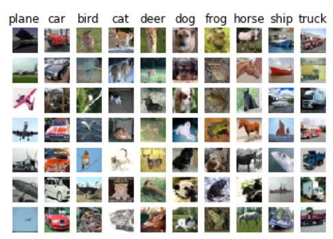
classes = ['plane', 'car', 'bird', 'cat', 'deer', 'dog', 'frog', 'horse', 'ship', 'truck']
num_classes = len(classes)
samples_per_class = 7
for y, cls in enumerate(classes):
    idxs = np.flatnonzero(y_train == y)
    idxs = np.random.choice(idxs, samples_per_class, replace=False)
    for i, idx in enumerate(idxs):
        plt_idx = i * num_classes + y + 1
        plt.subplot(samples_per_class, num_classes, plt_idx)
        plt.imshow(X_train[idx].astype('uint8'))
        plt.axis('off')
        if i == 0:
            plt.title(cls)
plt.show()

2. Data Preprocessing
Here we need to divide the data into a training set, a validation set, a test set, and a dev trial set, which is a small sample to test whether the program is working properly.We can't intersect the val test set and the train training set when we select the test set here to achieve a random effect.

# Split the data into train, val, and test sets. In addition we will
# create a small development set as a subset of the training data;
# we can use this for development so our code runs faster.
num_training = 49000
num_validation = 1000
num_test = 1000
num_dev = 500

# Our validation set will be num_validation points from the original
# training set.
mask = range(num_training, num_training + num_validation)
X_val = X_train[mask]
y_val = y_train[mask]

# Our training set will be the first num_train points from the original
# training set.
mask = range(num_training)
X_train = X_train[mask]
y_train = y_train[mask]

# We will also make a development set, which is a small subset of
# the training set.
mask = np.random.choice(num_training, num_dev, replace=False)
X_dev = X_train[mask]
y_dev = y_train[mask]

# We use the first num_test points of the original test set as our
# test set.
mask = range(num_test)
X_test = X_test[mask]
y_test = y_test[mask]

print('Train data shape: ', X_train.shape)
print('Train labels shape: ', y_train.shape)
print('Validation data shape: ', X_val.shape)
print('Validation labels shape: ', y_val.shape)
print('Test data shape: ', X_test.shape)
print('Test labels shape: ', y_test.shape)

Train data shape:  (49000, 32, 32, 3)
Train labels shape:  (49000,)
Validation data shape:  (1000, 32, 32, 3)
Validation labels shape:  (1000,)
Test data shape:  (1000, 32, 32, 3)
Test labels shape:  (1000,)

Next, we need to vectorize the data because our linear svm uses the matrix multiplication of Wx, where each column of W represents all the pixel templates of a category and each row of X represents the vectorized values of all the pixel points of each sample.

# Preprocessing: reshape the image data into rows
X_train = np.reshape(X_train, (X_train.shape[0], -1))
X_val = np.reshape(X_val, (X_val.shape[0], -1))
X_test = np.reshape(X_test, (X_test.shape[0], -1))
X_dev = np.reshape(X_dev, (X_dev.shape[0], -1))

# As a sanity check, print out the shapes of the data
print('Training data shape: ', X_train.shape)
print('Validation data shape: ', X_val.shape)
print('Test data shape: ', X_test.shape)
print('dev data shape: ', X_dev.shape)

Training data shape:  (49000, 3072)
Validation data shape:  (1000, 3072)
Test data shape:  (1000, 3072)
dev data shape:  (500, 3072)

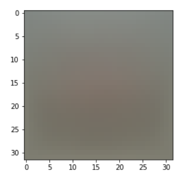
Next, let's show what the average of the pixel points of the training sample looks like.

# Preprocessing: subtract the mean image
# first: compute the image mean based on the training data
mean_image = np.mean(X_train, axis=0)
print(mean_image[:10]) # print a few of the elements
plt.figure(figsize=(4,4))
plt.imshow(mean_image.reshape((32,32,3)).astype('uint8')) # visualize the mean image
plt.show()

[130.64189 135.98174 132.47392 130.0557  135.34804 131.75401 130.96056
 136.14328 132.47636 131.48468]

Then all the training test samples are subtracted by such a pixel mean, the specific operation of this step is not very understood, but the statistical operations that often subtract the mean move the center point, which we can understand from this side, probably in order to make the center point of each dimension 0, and then reduce the degree of fitting, which is equivalent to reducing the degree of eigenvalue, reducing the calculationQuantity, refer to this link article here Differences between de-mean, whitening and centralization.

# second: subtract the mean image from train and test data
X_train -= mean_image
X_val -= mean_image
X_test -= mean_image
X_dev -= mean_image

Finally, add one more item for deviation.

# third: append the bias dimension of ones (i.e. bias trick) so that our SVM
# only has to worry about optimizing a single weight matrix W.
X_train = np.hstack([X_train, np.ones((X_train.shape[0], 1))])
X_val = np.hstack([X_val, np.ones((X_val.shape[0], 1))])
X_test = np.hstack([X_test, np.ones((X_test.shape[0], 1))])
X_dev = np.hstack([X_dev, np.ones((X_dev.shape[0], 1))])

print(X_train.shape, X_val.shape, X_test.shape, X_dev.shape)

(49000, 3073) (1000, 3073) (1000, 3073) (500, 3073)

3. Complete and run SVM
Here, if we run ipynb's SVM code in jupyter directly, we will output an exception because our SVM core code has not been written yet, so we need to open the linear_svm.py file to program the ToDo task. In this file, we have two tasks to complete, the first one is to use loops to program the gradient of w, the second is to use vector momentsThe matrix operation calculates the loss loss function and the gradient of W and outputs it.If a friend doesn't know what a gradient is, it can be interpreted as a partial derivative, so we know that one of the most traditional derivatives is to use the definition of the derivative, but this method requires updating one parameter at a time, which is very slow, so we can use the calculus to get the gradient, and then we assume the full text uses such a loss function.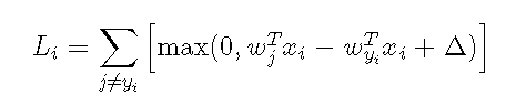

Here, delta means that when the prediction score function of the correct class is greater than that of the misplaced class, +1, we recognize that there is no loss in the prediction. This function means that when our first sample makes a prediction, each sample of i is predicted as the sum of the score of the wrong class and the correct class, +1, that is, the loss for the first sample.
So to find the gradient for this function, you just need to derive the corresponding w, and you get,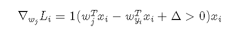

The above formula is a gradient calculation after misclassification, and 1 () is an exponential function that returns 1 if the parentheses condition is satisfied or 0 if it is not, that is, the gradient for the prediction error class is equal to the pixel value of the corresponding x.Then for the gradient of the correct predicted class, we update the weights in the opposite direction when we update the sum of all the losses predicted in class i. The intuitive understanding is that the larger the absolute skewness of the correct class, the stronger the weights need to be, because the prediction is too inaccurate without increasing the weights.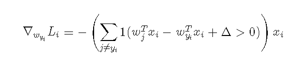

So this is our core formula for calculating the dW gradient. In fact, it is to determine if the score standard is greater than 0. If more than 0 pairs of error classes return Xi pairs of correct classes return -xi, so let's show you how this code is done.

import numpy as np
from random import shuffle
from past.builtins import xrange

def svm_loss_naive(W, X, y, reg):
  """
  Structured SVM loss function, naive implementation (with loops).

  Inputs have dimension D, there are C classes, and we operate on minibatches
  of N examples.

  Inputs:
  - W: A numpy array of shape (D, C) containing weights.
  - X: A numpy array of shape (N, D) containing a minibatch of data.
  - y: A numpy array of shape (N,) containing training labels; y[i] = c means
    that X[i] has label c, where 0 <= c < C.
  - reg: (float) regularization strength

  Returns a tuple of:
  - loss as single float
  - gradient with respect to weights W; an array of same shape as W
  """
  dW = np.zeros(W.shape) # initialize the gradient as zero

  # compute the loss and the gradient
  num_classes = W.shape[1]
  num_train = X.shape[0]
  loss = 0.0
  for i in xrange(num_train):
    scores = X[i].dot(W)
    correct_class_score = scores[y[i]]
    for j in xrange(num_classes):
      if j == y[i]:
        continue
      margin = scores[j] - correct_class_score + 1 # note delta = 1
      if margin > 0:
        loss += margin
        dW[:,j] += X[i].T
        dW[:,y[i]] -= X[i].T
  # Right now the loss is a sum over all training examples, but we want it
  # to be an average instead so we divide by num_train.
  loss /= num_train
  dW /= num_train
  # Add regularization to the loss.
  loss += reg * np.sum(W * W)
  dW += reg * W
  #############################################################################
  # TODO:                                                                     #
  # Compute the gradient of the loss function and store it dW.                #
  # Rather that first computing the loss and then computing the derivative,   #
  # it may be simpler to compute the derivative at the same time that the     #
  # loss is being computed. As a result you may need to modify some of the    #
  # code above to compute the gradient.                                       #
  #############################################################################


  return loss, dW


def svm_loss_vectorized(W, X, y, reg):
  """
  Structured SVM loss function, vectorized implementation.

  Inputs and outputs are the same as svm_loss_naive.
  """
  loss = 0.0
  dW = np.zeros(W.shape) # initialize the gradient as zero

  #############################################################################
  # TODO:                                                                     #
  # Implement a vectorized version of the structured SVM loss, storing the    #
  # result in loss.                                                           #
  #############################################################################
  pass
  num_train = X.shape[0]
  scores = np.dot(X, W)
  correct_class_score = scores[range(num_train), list(y)].reshape(-1, 1)#Become column
  margin = np.maximum(0, scores - correct_class_score + 1)
  margin[range(num_train), list(y)] = 0
  loss = np.sum(margin)/num_train + reg * np.sum(W*W)
  #############################################################################
  #                             END OF YOUR CODE                              #
  #############################################################################


  #############################################################################
  # TODO:                                                                     #
  # Implement a vectorized version of the gradient for the structured SVM     #
  # loss, storing the result in dW.                                           #
  #                                                                           #
  # Hint: Instead of computing the gradient from scratch, it may be easier    #
  # to reuse some of the intermediate values that you used to compute the     #
  # loss.                                                                     #
  #############################################################################
  pass
  num_class = W.shape[1]
  m = np.zeros((num_train, num_class))
  m[margin > 0] = 1
  m[range(num_train), list(y)] = 0
  m[range(num_train), list(y)] = -np.sum(m, axis=1)
  dW = np.dot(X.T, m)/num_train + reg * W

  #############################################################################
  #                             END OF YOUR CODE                              #
  #############################################################################

  return loss, dW

The code accomplishes three tasks that need to be done in this article. It is worth noting that we need to add a reg regular item to both the calculated dw and loss to avoid overfitting them.
So let's run the job code and see what happens.

# Evaluate the naive implementation of the loss we provided for you:
from cs231n.classifiers.linear_svm import svm_loss_naive
import time

# generate a random SVM weight matrix of small numbers
W = np.random.randn(3073, 10) * 0.0001 

loss, grad = svm_loss_naive(W, X_dev, y_dev, 0.000005)
print('loss: %f' % (loss, ))

The first step is to derive the loss function from the svm's general loop calculation, which does not require us to write anything.

loss: 9.035526

Then running the next code will test if the loss function we write is correct. One criterion is to compare the solution we get from the calculus with the solution defined by the derivative. If the difference is small, the calculation is correct.

# Once you've implemented the gradient, recompute it with the code below
# and gradient check it with the function we provided for you
from cs231n.classifiers.linear_svm import svm_loss_naive
import time
# Compute the loss and its gradient at W.
loss, grad = svm_loss_naive(W, X_dev, y_dev, 0.0)

# Numerically compute the gradient along several randomly chosen dimensions, and
# compare them with your analytically computed gradient. The numbers should match
# almost exactly along all dimensions.
from cs231n.gradient_check import grad_check_sparse
f = lambda w: svm_loss_naive(w, X_dev, y_dev, 0.0)[0]
grad_numerical = grad_check_sparse(f, W, grad)

# do the gradient check once again with regularization turned on
# you didn't forget the regularization gradient did you?
loss, grad = svm_loss_naive(W, X_dev, y_dev, 5e1)
f = lambda w: svm_loss_naive(w, X_dev, y_dev, 5e1)[0]
grad_numerical = grad_check_sparse(f, W, grad)

numerical: -11.134769 analytic: -11.134769, relative error: 7.492919e-12
numerical: -26.201969 analytic: -26.201969, relative error: 2.276806e-11
numerical: 17.007888 analytic: 17.007888, relative error: 8.322863e-12
numerical: 24.357402 analytic: 24.357402, relative error: 3.966234e-12
numerical: 11.060589 analytic: 11.060589, relative error: 1.475823e-11
numerical: 14.618717 analytic: 14.618717, relative error: 6.643635e-12
numerical: -28.965377 analytic: -28.965377, relative error: 1.620809e-12
numerical: -12.924270 analytic: -12.924270, relative error: 1.946887e-12
numerical: -37.095280 analytic: -37.095280, relative error: 3.942003e-12
numerical: 16.260672 analytic: 16.260672, relative error: 4.586001e-13
numerical: -35.859216 analytic: -35.862116, relative error: 4.042911e-05
numerical: -0.298664 analytic: -0.288489, relative error: 1.732885e-02
numerical: 20.924849 analytic: 20.921766, relative error: 7.368654e-05
numerical: 15.027211 analytic: 15.025921, relative error: 4.291960e-05
numerical: 6.215818 analytic: 6.223036, relative error: 5.802678e-04
numerical: 0.161299 analytic: 0.156143, relative error: 1.624406e-02
numerical: -9.542728 analytic: -9.541662, relative error: 5.582052e-05
numerical: 3.184572 analytic: 3.178109, relative error: 1.015709e-03
numerical: 7.230887 analytic: 7.239002, relative error: 5.608088e-04
numerical: 37.075271 analytic: 37.067189, relative error: 1.090062e-04

We can see that the loss of numericla and analytic calculations are very close, so we think there is no problem with programming, but there is another problem. Why the results of the two calculations are still slightly different? This problem will be left for analysis in the next series of thinking questions.
Next, we need to use the matrix operation just written to calculate loss and dw functions. In fact, the idea of matrix operation is a whole operation, which integrates for loop into a whole operation, but the details of implementation may require programming attention.

# Next implement the function svm_loss_vectorized; for now only compute the loss;
# we will implement the gradient in a moment.
tic = time.time()
loss_naive, grad_naive = svm_loss_naive(W, X_dev, y_dev, 0.000005)
toc = time.time()
print('Naive loss: %e computed in %fs' % (loss_naive, toc - tic))
print(loss)

Naive loss: 9.138494e+00 computed in 0.092990s
9.15405317783763

from cs231n.classifiers.linear_svm import svm_loss_vectorized
tic = time.time()
loss_vectorized, _ = svm_loss_vectorized(W, X_dev, y_dev, 0.000005)
toc = time.time()
print('Vectorized loss: %e computed in %fs' % (loss_vectorized, toc - tic))
print(loss_vectorized)
# The losses should match but your vectorized implementation should be much faster.
print(loss_naive - loss_vectorized)

Vectorized loss: 9.138494e+00 computed in 0.001954s
9.138493682409688
2.4868995751603507e-14

You can see that the difference between the result of vector calculation and the result of for loop is very small, which may be caused by the different storage precision.Of course, we compare loss better because we use the F-norm to compare the gradients calculated by the two methods for a single value.

# Complete the implementation of svm_loss_vectorized, and compute the gradient
# of the loss function in a vectorized way.

# The naive implementation and the vectorized implementation should match, but
# the vectorized version should still be much faster.
tic = time.time()
_, grad_naive = svm_loss_naive(W, X_dev, y_dev, 0.000005)
toc = time.time()

print('Naive loss and gradient: computed in %fs' % (toc - tic))

tic = time.time()
_, grad_vectorized = svm_loss_vectorized(W, X_dev, y_dev, 0.000005)
toc = time.time()

print('Vectorized loss and gradient: computed in %fs' % (toc - tic))

# The loss is a single number, so it is easy to compare the values computed
# by the two implementations. The gradient on the other hand is a matrix, so
# we use the Frobenius norm to compare them.
difference = np.linalg.norm(grad_naive - grad_vectorized, ord='fro')
print('difference: %f' % difference)

Vectorized loss and gradient: computed in 0.015625s
difference: 0.000000

You can see that there is also little difference, and vector operations are computed faster.Of course, even if the speed of calculation is faster, when we face a lot of data, if we calculate all the data each time, or book updates the weight through all the data, it will undoubtedly greatly increase the burden of calculation. To solve this problem, we use SGD, which is also called random gradient descent. The difference between this method and gradient descent is random. The main idea is as follows:It's the idea of randomly removing 200 rows of data from 5,000 rows (numpy.random.choice implements this idea) and iterating over local data, then selecting 2,000 times so that you can quickly calculate and update weights with small-scale data, then you'll move on to the train function in another file, linear_classifier.py, filled with random gradientsThe downward core function, and all we need to do is implement random data collection.Then there is one more thing to do to predict the categories of our train data based on the final W.The code is as follows.

from __future__ import print_function

import numpy as np
from cs231n.classifiers.linear_svm import *
from cs231n.classifiers.softmax import *
from past.builtins import xrange


class LinearClassifier(object):

  def __init__(self):
    self.W = None

  def train(self, X, y, learning_rate=1e-3, reg=1e-5, num_iters=100,
            batch_size=200, verbose=False):
    """
    Train this linear classifier using stochastic gradient descent.

    Inputs:
    - X: A numpy array of shape (N, D) containing training data; there are N
      training samples each of dimension D.
    - y: A numpy array of shape (N,) containing training labels; y[i] = c
      means that X[i] has label 0 <= c < C for C classes.
    - learning_rate: (float) learning rate for optimization.
    - reg: (float) regularization strength.
    - num_iters: (integer) number of steps to take when optimizing
    - batch_size: (integer) number of training examples to use at each step.
    - verbose: (boolean) If true, print progress during optimization.

    Outputs:
    A list containing the value of the loss function at each training iteration.
    """
    num_train, dim = X.shape
    num_classes = np.max(y) + 1 # assume y takes values 0...K-1 where K is number of classes
    if self.W is None:
      # lazily initialize W
      self.W = 0.001 * np.random.randn(dim, num_classes)

    # Run stochastic gradient descent to optimize W
    loss_history = []
    for it in xrange(num_iters):
      index = np.random.choice(num_train, batch_size, replace=True)
      X_batch = X[index]
      y_batch = y[index]

      #########################################################################
      # TODO:                                                                 #
      # Sample batch_size elements from the training data and their           #
      # corresponding labels to use in this round of gradient descent.        #
      # Store the data in X_batch and their corresponding labels in           #
      # y_batch; after sampling X_batch should have shape (dim, batch_size)   #
      # and y_batch should have shape (batch_size,)                           #
      #                                                                       #
      # Hint: Use np.random.choice to generate indices. Sampling with         #
      # replacement is faster than sampling without replacement.              #
      #########################################################################
      pass
      #########################################################################
      #                       END OF YOUR CODE                                #
      #########################################################################

      # evaluate loss and gradient
      loss, grad = self.loss(X_batch, y_batch, reg)
      loss_history.append(loss)
      self.W += -learning_rate * grad
      # perform parameter update
      #########################################################################
      # TODO:                                                                 #
      # Update the weights using the gradient and the learning rate.          #
      #########################################################################
      pass
      #########################################################################
      #                       END OF YOUR CODE                                #
      #########################################################################

      if verbose and it % 100 == 0:
        print('iteration %d / %d: loss %f' % (it, num_iters, loss))

    return loss_history

  def predict(self, X):
    """
    Use the trained weights of this linear classifier to predict labels for
    data points.

    Inputs:
    - X: A numpy array of shape (N, D) containing training data; there are N
      training samples each of dimension D.

    Returns:
    - y_pred: Predicted labels for the data in X. y_pred is a 1-dimensional
      array of length N, and each element is an integer giving the predicted
      class.
    """
    y_pred = np.zeros(X.shape[0])
    scores = np.dot(X, self.W)
    y_pred = np.argmax(scores, axis=1)
    ###########################################################################
    # TODO:                                                                   #
    # Implement this method. Store the predicted labels in y_pred.            #
    ###########################################################################
    pass
    ###########################################################################
    #                           END OF YOUR CODE                              #
    ###########################################################################
    return y_pred
  
  def loss(self, X_batch, y_batch, reg):
    """
    Compute the loss function and its derivative. 
    Subclasses will override this.

    Inputs:
    - X_batch: A numpy array of shape (N, D) containing a minibatch of N
      data points; each point has dimension D.
    - y_batch: A numpy array of shape (N,) containing labels for the minibatch.
    - reg: (float) regularization strength.

    Returns: A tuple containing:
    - loss as a single float
    - gradient with respect to self.W; an array of the same shape as W
    """
    pass


class LinearSVM(LinearClassifier):
  """ A subclass that uses the Multiclass SVM loss function """

  def loss(self, X_batch, y_batch, reg):
    return svm_loss_vectorized(self.W, X_batch, y_batch, reg)


class Softmax(LinearClassifier):
  """ A subclass that uses the Softmax + Cross-entropy loss function """

  def loss(self, X_batch, y_batch, reg):
    return softmax_loss_vectorized(self.W, X_batch, y_batch, reg)

Let's run the job code and see the results.

# In the file linear_classifier.py, implement SGD in the function
# LinearClassifier.train() and then run it with the code below.

from cs231n.classifiers import LinearSVM
svm = LinearSVM()
tic = time.time()
loss_hist = svm.train(X_train, y_train, learning_rate=1e-7, reg=2.5e4,
                      num_iters=2000, verbose=True)
toc = time.time()
print('That took %fs' % (toc - tic))

iteration 0 / 2000: loss 785.193662
iteration 100 / 2000: loss 469.951361
iteration 200 / 2000: loss 285.152670
iteration 300 / 2000: loss 173.940086
iteration 400 / 2000: loss 106.734203
iteration 500 / 2000: loss 66.067783
iteration 600 / 2000: loss 41.010264
iteration 700 / 2000: loss 27.581060
iteration 800 / 2000: loss 18.393378
iteration 900 / 2000: loss 12.956286
iteration 1000 / 2000: loss 10.400926
iteration 1100 / 2000: loss 8.312311
iteration 1200 / 2000: loss 6.956938
iteration 1300 / 2000: loss 6.775997
iteration 1400 / 2000: loss 5.950798
iteration 1500 / 2000: loss 5.256139
iteration 1600 / 2000: loss 5.524237
iteration 1700 / 2000: loss 5.749462
iteration 1800 / 2000: loss 6.222899
iteration 1900 / 2000: loss 5.239182
That took 9.655279s

You can see that as the number of iterations increases, the overall loss function decreases, that is, the prediction accuracy increases.Let's take a look at the drawing below.

# A useful debugging strategy is to plot the loss as a function of
# iteration number:
plt.plot(loss_hist)
plt.xlabel('Iteration number')
plt.ylabel('Loss value')
plt.show()

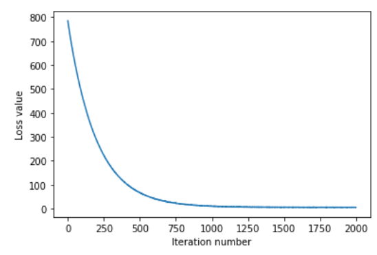
So you can see that as the number of iterations increases, the size of the loss function decreases rapidly and tends to stabilize. Let's see how accurate the predictions for train and val data are.

# Write the LinearSVM.predict function and evaluate the performance on both the
# training and validation set
y_train_pred = svm.predict(X_train)
print('training accuracy: %f' % (np.mean(y_train == y_train_pred), ))
y_val_pred = svm.predict(X_val)
print('validation accuracy: %f' % (np.mean(y_val == y_val_pred), ))

training accuracy: 0.376714
validation accuracy: 0.388000

Accuracy at 0.37 and 0.38 is generally not good, but for linear svm the results are OK.Finally, cross-validation is used to select the best parameters. Here we train train data with different parameters, then validate the data, and select the most accurate set of parameters to be substituted for test to output the final result.
The last task here is to complete the code for cross-validation. The main idea is to cycle through different parameters to make predictions, then keep updating the most accurate parameters.The code is as follows.

# Use the validation set to tune hyperparameters (regularization strength and
# learning rate). You should experiment with different ranges for the learning
# rates and regularization strengths; if you are careful you should be able to
# get a classification accuracy of about 0.4 on the validation set.

learning_rates = [1.4e-7, 1.5e-7, 1.6e-7]
regularization_strengths = [8000.0, 9000.0, 10000.0, 11000.0, 18000.0, 19000.0, 20000.0, 21000.0]

# results is dictionary mapping tuples of the form
# (learning_rate, regularization_strength) to tuples of the form
# (training_accuracy, validation_accuracy). The accuracy is simply the fraction
# of data points that are correctly classified.
results = {}
best_lr = None
best_reg = None
best_val = -1   # The highest validation accuracy that we have seen so far.
best_svm = None # The LinearSVM object that achieved the highest validation rate.
for lr in learning_rates:
    for reg in regularization_strengths:
        svm = LinearSVM()
        loss_history = svm.train(X_train, y_train, learning_rate = lr, reg = reg, num_iters = 5000)
        y_train_pred = svm.predict(X_train)
        accuracy_train = np.mean(y_train_pred == y_train)
        y_val_pred = svm.predict(X_val)
        accuracy_val = np.mean(y_val_pred == y_val)
        if accuracy_val > best_val:
            best_lr = lr
            best_reg = reg
            best_val = accuracy_val
            best_svm = svm
        results[(lr, reg)] = accuracy_train, accuracy_val
        
################################################################################
# TODO:                                                                        #
# Write code that chooses the best hyperparameters by tuning on the validation #
# set. For each combination of hyperparameters, train a linear SVM on the      #
# training set, compute its accuracy on the training and validation sets, and  #
# store these numbers in the results dictionary. In addition, store the best   #
# validation accuracy in best_val and the LinearSVM object that achieves this  #
# accuracy in best_svm.                                                        #
#                                                                              #
# Hint: You should use a small value for num_iters as you develop your         #
# validation code so that the SVMs don't take much time to train; once you are #
# confident that your validation code works, you should rerun the validation   #
# code with a larger value for num_iters.                                      #
################################################################################
pass
################################################################################
#                              END OF YOUR CODE                                #
################################################################################
    
# Print out results.
for lr, reg in sorted(results):
    train_accuracy, val_accuracy = results[(lr, reg)]
    print('lr %e reg %e train accuracy: %f val accuracy: %f' % (
                lr, reg, train_accuracy, val_accuracy))
    
print('best validation accuracy achieved during cross-validation: %f' % best_val)

lr 1.400000e-07 reg 8.000000e+03 train accuracy: 0.399837 val accuracy: 0.402000
lr 1.400000e-07 reg 9.000000e+03 train accuracy: 0.391000 val accuracy: 0.396000
lr 1.400000e-07 reg 1.000000e+04 train accuracy: 0.392224 val accuracy: 0.393000
lr 1.400000e-07 reg 1.100000e+04 train accuracy: 0.391837 val accuracy: 0.392000
lr 1.400000e-07 reg 1.800000e+04 train accuracy: 0.383347 val accuracy: 0.393000
lr 1.400000e-07 reg 1.900000e+04 train accuracy: 0.377673 val accuracy: 0.373000
lr 1.400000e-07 reg 2.000000e+04 train accuracy: 0.383551 val accuracy: 0.386000
lr 1.400000e-07 reg 2.100000e+04 train accuracy: 0.383347 val accuracy: 0.385000
lr 1.500000e-07 reg 8.000000e+03 train accuracy: 0.394367 val accuracy: 0.390000
lr 1.500000e-07 reg 9.000000e+03 train accuracy: 0.392653 val accuracy: 0.393000
lr 1.500000e-07 reg 1.000000e+04 train accuracy: 0.393878 val accuracy: 0.402000
lr 1.500000e-07 reg 1.100000e+04 train accuracy: 0.385612 val accuracy: 0.365000
lr 1.500000e-07 reg 1.800000e+04 train accuracy: 0.382837 val accuracy: 0.393000
lr 1.500000e-07 reg 1.900000e+04 train accuracy: 0.377633 val accuracy: 0.386000
lr 1.500000e-07 reg 2.000000e+04 train accuracy: 0.383571 val accuracy: 0.383000
lr 1.500000e-07 reg 2.100000e+04 train accuracy: 0.384469 val accuracy: 0.382000
lr 1.600000e-07 reg 8.000000e+03 train accuracy: 0.393816 val accuracy: 0.390000
lr 1.600000e-07 reg 9.000000e+03 train accuracy: 0.394673 val accuracy: 0.394000
lr 1.600000e-07 reg 1.000000e+04 train accuracy: 0.392776 val accuracy: 0.392000
lr 1.600000e-07 reg 1.100000e+04 train accuracy: 0.387388 val accuracy: 0.383000
lr 1.600000e-07 reg 1.800000e+04 train accuracy: 0.383143 val accuracy: 0.393000
lr 1.600000e-07 reg 1.900000e+04 train accuracy: 0.381224 val accuracy: 0.390000
lr 1.600000e-07 reg 2.000000e+04 train accuracy: 0.379959 val accuracy: 0.387000
lr 1.600000e-07 reg 2.100000e+04 train accuracy: 0.375388 val accuracy: 0.397000
best validation accuracy achieved during cross-validation: 0.402000

# Visualize the cross-validation results
import math
x_scatter = [math.log10(x[0]) for x in results]
y_scatter = [math.log10(x[1]) for x in results]

# plot training accuracy
marker_size = 100
colors = [results[x][0] for x in results]
plt.subplot(2, 1, 1)
plt.scatter(x_scatter, y_scatter, marker_size, c=colors)
plt.colorbar()
plt.xlabel('log learning rate')
plt.ylabel('log regularization strength')
plt.title('CIFAR-10 training accuracy')

# plot validation accuracy
colors = [results[x][1] for x in results] # default size of markers is 20
plt.subplot(2, 1, 2)
plt.scatter(x_scatter, y_scatter, marker_size, c=colors)
plt.colorbar()
plt.xlabel('log learning rate')
plt.ylabel('log regularization strength')
plt.title('CIFAR-10 validation accuracy')
plt.show()

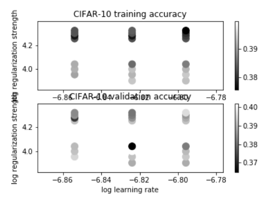
The fluctuations of prediction accuracy under different parameters are shown. Let's take a look at the prediction accuracy of test using the optimal parameters.

# Evaluate the best svm on test set
y_test_pred = best_svm.predict(X_test)
test_accuracy = np.mean(y_test == y_test_pred)
print('linear SVM on raw pixels final test set accuracy: %f' % test_accuracy)

linear SVM on raw pixels final test set accuracy: 0.377000

The prediction accuracy is 0.37, which is similar to the training set. As to whether the prediction is more accurate or not, we can see from the previous loss function graph that we need to increase a large number of iterations in the future to improve the accuracy slightly, so it is not cost-effective, so we think this prediction result is reasonable.
Finally, we will show the W we trained visually to see what we trained after half a day. The explanation course for W says that it is a template for each category. When a sample is entered and multiplied with the template to get a corresponding score, the high score indicates that you fit all parts of the template well.

# Visualize the learned weights for each class.
# Depending on your choice of learning rate and regularization strength, these may
# or may not be nice to look at.
w = best_svm.W[:-1,:] # strip out the bias
w = w.reshape(32, 32, 3, 10)
w_min, w_max = np.min(w), np.max(w)
classes = ['plane', 'car', 'bird', 'cat', 'deer', 'dog', 'frog', 'horse', 'ship', 'truck']
for i in range(10):
    plt.subplot(2, 5, i + 1)
      
    # Rescale the weights to be between 0 and 255
    wimg = 255.0 * (w[:, :, :, i].squeeze() - w_min) / (w_max - w_min)
    plt.imshow(wimg.astype('uint8'))
    plt.axis('off')
    plt.title(classes[i])

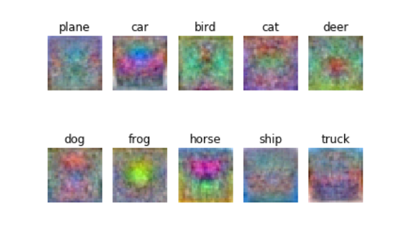
This picture can show that horse is the two-headed horse that we talked about in the class.

epilogue
This time, we have a preliminary understanding of the classification implementation of linear svm, and we will continue to update this series later.
Thank you for reading.
Reference resources
cs231n svm course assignments red stone