In early 2019, ApacheCN volunteers translated the Chinese version of PyTorch 1.0 ( github address ) and has been officially authorized by PyTorch, and I believe there are already many people who are Chinese Documents Official Web I saw it on.But for now Proofreading There is still a shortage of staff, and we hope you will take part in it.Bruce Lin g, who is responsible for PyTorch, has been having email conversations for some time.In the future, when appropriate, we will organize volunteers to do other PyTorch projects, welcome you to join us and follow us.We hope that our series of work can help you all.
A torch.nn packet can be used to construct a neural network.
We have introduced autograd, and NN packages rely on autograd packages to define models and derive them.A nn.Module contains layers and a forward(input) method that returns output.
For example, the following neural network can classify numbers: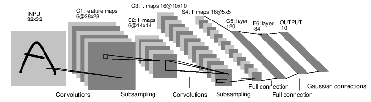
This is a simple feed-forward network.It accepts an input, then feeds it into the next layer, transfers it layer by layer, and finally gives the output.
A typical training process for a neural network is as follows:
- Define a neural network that contains some learnable parameters (or weights)
- Iterate over the input dataset
- Processing inputs over the network
- Calculate loss (distance between output and correct answer)
- Parameters that propagate gradients back to the network
- Updating the weights of a network generally uses a simple rule: weight = weight - learning_rate * gradient
Define Network
Let's define such a network:
import torch
import torch.nn as nn
import torch.nn.functional as F


class Net(nn.Module):

    def __init__(self):
        super(Net, self).__init__()
        # Input image channel:1; Output channel:6; 5x5 convolution kernel
        self.conv1 = nn.Conv2d(1, 6, 5)
        self.conv2 = nn.Conv2d(6, 16, 5)
        # an affine operation: y = Wx + b
        self.fc1 = nn.Linear(16 * 5 * 5, 120)
        self.fc2 = nn.Linear(120, 84)
        self.fc3 = nn.Linear(84, 10)

    def forward(self, x):
        # 2x2 Max pooling
        x = F.max_pool2d(F.relu(self.conv1(x)), (2, 2))
        # If it's a square matrix, you can define it with only one number
        x = F.max_pool2d(F.relu(self.conv2(x)), 2)
        x = x.view(-1, self.num_flat_features(x))
        x = F.relu(self.fc1(x))
        x = F.relu(self.fc2(x))
        x = self.fc3(x)
        return x

    def num_flat_features(self, x):
        size = x.size()[1:]  # All other dimensions except batch dimension
        num_features = 1
        for s in size:
            num_features *= s
        return num_features


net = Net()
print(net)
Output:
Net(
  (conv1): Conv2d(1, 6, kernel_size=(5, 5), stride=(1, 1))
  (conv2): Conv2d(6, 16, kernel_size=(5, 5), stride=(1, 1))
  (fc1): Linear(in_features=400, out_features=120, bias=True)
  (fc2): Linear(in_features=120, out_features=84, bias=True)
  (fc3): Linear(in_features=84, out_features=10, bias=True)
)
We just need to define the forward function, which is automatically defined when autograd is used, and the backward function is used to calculate the derivative.Any operation and calculation on a tensor can be used in the forward function.
The learnable parameters of a model can be returned through net.parameters()
params = list(net.parameters())
print(len(params))
print(params[0].size())  # conv1's .weight
Output:
10
torch.Size([6, 1, 5, 5])
Let's try a random 32x32 input.Note: The expected input for this network (LeNet) is 32x32.If you use an MNIST dataset to train this network, resize the picture to 32x32.
input = torch.randn(1, 1, 32, 32)
out = net(input)
print(out)
Output:
tensor([[ 0.0399, -0.0856,  0.0668,  0.0915,  0.0453, -0.0680, -0.1024,  0.0493,
         -0.1043, -0.1267]], grad_fn=<AddmmBackward>)
Clear the gradient cache for all parameters and then reverse propagate the random gradient:
net.zero_grad()
out.backward(torch.randn(1, 10))
Be careful:
Torch.nn only supports mini-batches.The entire torch.nn package only supports input of small batches of samples, not individual samples.
For example, nn.Conv2d accepts a four-dimensional tensor, nSamples x nChannels x Height x Width
If it's a separate sample, simply use input.unsqueeze(0) to add a "false" batch size dimension.
Before proceeding, let's review all the classes we've seen so far.
Review:
-
torch.Tensor - A multidimensional array that supports automatic derivation operations such as backward(), while preserving gradients for tensors.
-
nn.Module - Neural network module.It is a convenient way to encapsulate parameters, with functions such as moving parameters to GPU, exporting, loading, etc.
-
nn.Parameter - A type of tensor that is automatically registered as a parameter when assigned to a Module as an attribute.
-
autograd.Function - Implements the definition of auto-derivative forward and reverse propagation, where each Tensor creates at least one Function node that connects to the function that created the Tensor and codes its history.
So far, we have discussed:
- Define a neural network
- Processing Input Call backward
There are still:
- Calculate loss
- Update Network Weights
loss function
A loss function accepts a pair of outputs (targets) as input and calculates a value to estimate how much the network output differs from the target value.
There are many different nn packages loss function .nn.MSELoss is a simpler method of calculating mean-squared error s for output and target.
For example:
output = net(input)
target = torch.randn(10)  # Using simulated data in this example
target = target.view(1, -1)  # Make the target value consistent with the shape of the data value
criterion = nn.MSELoss()

loss = criterion(output, target)
print(loss)
Output:
tensor(1.0263, grad_fn=<MseLossBackward>)
Now, if you use loss's.grad_fn attribute to track the reverse propagation process, you can see the following calculation diagram:
input -> conv2d -> relu -> maxpool2d -> conv2d -> relu -> maxpool2d
      -> view -> linear -> relu -> linear -> relu -> linear
      -> MSELoss
      -> loss
So when we call loss.backward(), the whole graph begins with a loss differential, where all the.Grad properties with the required_grad=True tensor set accumulate the gradient tensor.
To illustrate this, let's go back a few steps:
print(loss.grad_fn)  # MSELoss
print(loss.grad_fn.next_functions[0][0])  # Linear
print(loss.grad_fn.next_functions[0][0].next_functions[0][0])  # ReLU
Output:
<MseLossBackward object at 0x7f94c821fdd8>
<AddmmBackward object at 0x7f94c821f6a0>
<AccumulateGrad object at 0x7f94c821f6a0>
Reverse Propagation
We only need to call loss.backward() to reverse propagate weights.We need to clear the existing gradient, otherwise the gradient will add up with the existing gradient.
Now we'll call loss.backward() and look at the gradient of the bias of the conv1 layer before and after reverse propagation.
net.zero_grad()     # Clear the gradient cache for all parameter s

print('conv1.bias.grad before backward')
print(net.conv1.bias.grad)

loss.backward()

print('conv1.bias.grad after backward')
print(net.conv1.bias.grad)
Output:
conv1.bias.grad before backward
tensor([0., 0., 0., 0., 0., 0.])
conv1.bias.grad after backward
tensor([ 0.0084,  0.0019, -0.0179, -0.0212,  0.0067, -0.0096])
Now we've seen how to use the loss function.
Read Later
Neural network packages contain modules and loss functions that form the building blocks of deep neural networks.For a complete list of documents, see Here.
The only thing to learn now is:
- Update the weight of the network
Update Weights
The simplest update rule is the random gradient descent (SGD):
weight = weight - learning_rate * gradient
We can do this using simple python code:
learning_rate = 0.01
for f in net.parameters():
    f.data.sub_(f.grad.data * learning_rate)
However, when using neural networks, you may want to use a variety of different update rules, such as SGD, Nesterov-SGD, Adam, RMSProp, and so on.To do this, we built a smaller package, torch.optim, that implements all these methods.It's easy to use it:
import torch.optim as optim

# Create optimizer
optimizer = optim.SGD(net.parameters(), lr=0.01)

# In the iteration of training:
optimizer.zero_grad()   # Zero Gradient Cache
output = net(input)
loss = criterion(output, target)
loss.backward()
optimizer.step()    # Update parameters
Be careful:
Observe how gradient caches are manually zeroed out using optimizer.zero_grad().This is because gradients are cumulative, as before Reverse Propagation Chapter As described.
m.SGD(net.parameters(), lr=0.01)
In the iteration of training:
optimizer.zero_grad() #Zero Gradient Cache
output = net(input)
loss = criterion(output, target)
loss.backward()
optimizer.step()#Update parameters
>Note:
>
>Watch how the gradient cache is manually zeroed out using `optimizer.zero_grad()'.This is because gradients are cumulative, as described in the previous [Reverse Propagation Chapter] (#Reverse Propagation).