Pan Chuang AI sharing
Author amitvkulkarni
Compile | Flin
Source | analyticsvidhya
[guide] "if you don't care about your customers, your competitors will care" -- Bob Hooey
summary
Customer lifetime value is the profit that an enterprise obtains from a specific customer during the period when a specific customer is associated with the enterprise. Each industry has its own set of indicators, which can be tracked and measured to help enterprises target the right customers and predict the future customer base.
CLV enables various departments such as marketing and sales to plan their strategies and provide specific products or customized services to the most valuable customers. It also provides a framework for customer service teams to understand the efforts needed to develop and retain customers.
When CLV is applied together with other tools (such as customer segmentation, pricing and marketing strategy), it is the most effective and adds great value, which means that it tells us who our most profitable customers are, but it doesn't tell us which products need to be sold at what price and quantity.
Therefore, CLV should be applied wisely, not as the only standard for making business decisions. CLV may change according to the business model and its objectives, which means that its definition and calculation need to be reviewed regularly.
The following is how CLV is used in various industries
Insurance: the marketing team wants to know which customers are most likely to pay high premiums rather than claims, which in turn helps them acquire new customers and grow their business.
Telecom: the predicted CLV is used to understand the likelihood of current customer loyalty and their continued use of programs or subscriptions.
Retail: CLV is used to understand purchase behavior and consume for specific customers with customized offers / discounts.
Benefits of CLV
- Acquisition cost: help determine acceptable acquisition cost and where to put the marketing work
- Prospects: help determine the future value of existing and potential new customers
- Customer relationship: be able to establish a stronger and effective relationship with customers
- Brand loyalty: good relationships help build brand loyalty
target
We will explore the following steps and, at the end of this blog, build a customer lifetime value simulator application using plot dash.
- Customer lifetime value (CLV) overview
- Benefits of CLV
- Data exploration
- CLV calculation
- Developing applications using Plotly dash
- Conclusion
introduction
We will use the machine learning repository from UCI( https://archive.ics.uci.edu/ml/datasets/online+retail) to build Python applications.
The property description can be found in the URL above.
Let's load the dataset and view the data.
data = pd.read_excel("./data/Online_Retail.xlsx")
data.head(10)
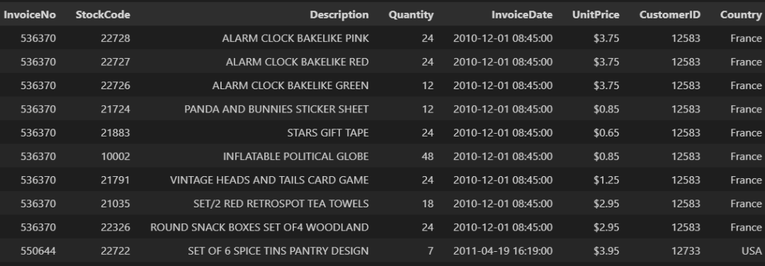
data.info()
Data columns (total 8 columns):
 #   Column       Non-Null Count  Dtype
---  ------       --------------  -----
 0   InvoiceNo    40 non-null     int64
 1   StockCode    40 non-null     object
 2   Description  40 non-null     object
 3   Quantity     40 non-null     int64
 4   InvoiceDate  40 non-null     datetime64[ns]
 5   UnitPrice    40 non-null     float64
 6   CustomerID   40 non-null     int64
 7   Country      40 non-null     object
dtypes: datetime64[ns](1), float64(1), int64(3), object(3)
Data preprocessing
Let's clean up the data and create the new functions we need to calculate the CLV at a later stage.
- Data cleaning: delete duplicate records
- Quantity: we will only consider positive quantity. Any negative value means that the product is returned for some reason.
- Total purchase: this will be the unit price x quantity of the product
- Aggregation: since the data is at the transaction level, we aggregate the data by CustomerID and Country. We will do this by using the group by function.
- Average order value: this will be the ratio of the amount spent to the number of transactions
- Purchase frequency: This is the ratio of the total number of transactions to the total number of transactions. It is the average number of orders per customer.
- Churn rate: This is the percentage of customers who have not reordered.
- CLTV: (average order value x purchase frequency) / turnover rate)
- In addition, let's rename some column names to make them easy to track.
After completing the above steps, the data will be as follows.
As we progress, we will further address this issue.

The complete code can be obtained from pre-processing.py: https://github.com/amitvkulkarni/Data-Apps/blob/main/Customer%20Lifetime%20Value/pre_processing.py
Developing applications using Plotly Dash
We will use plot dash to develop our application, a Python framework for building data applications. Let's create a file called app.py and start by loading the library.
Step 1: load the library
import pandas as pd
import matplotlib.pyplot as plt
import seaborn as sns
import datetime as dt
import numpy as np
import dash
import dash_table
import dash_core_components as dcc
import dash_html_components as html
from dash.dependencies import Input, Output, State
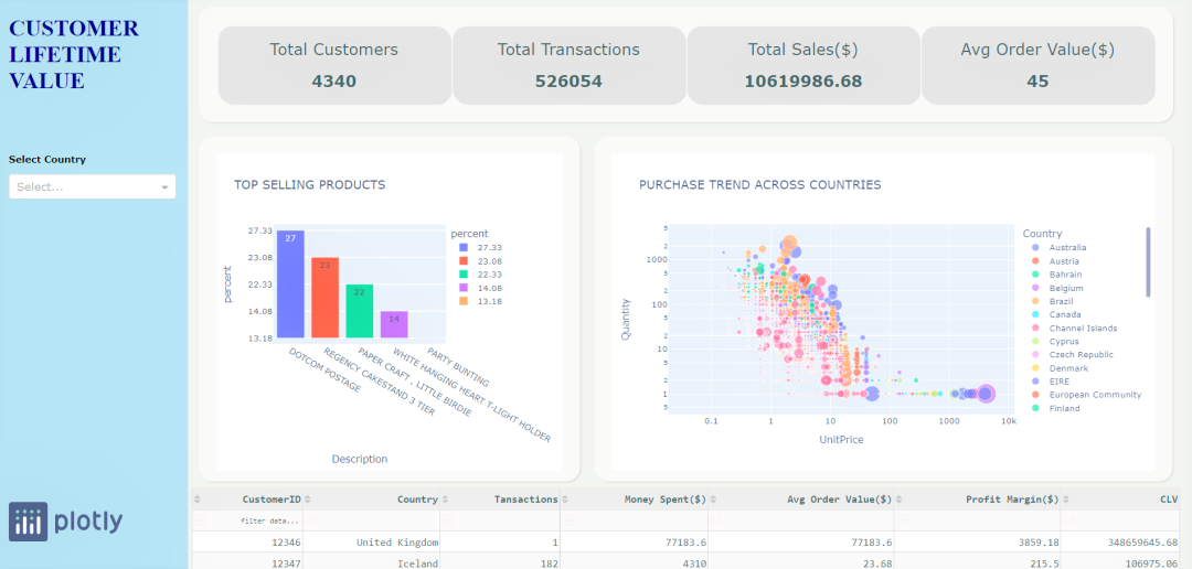
Step 2: design layout (UI)
Card: all 4 KPI s we are tracking will be at the top of the page. Defines font size, color, etc. In addition, the unique ID of each card will later be used to populate the value.
html.H2('Total Customers', style={
    'font-weight': 'normal'}),
html.H2(id='id_total_customer', style = {'color': 'DarkSlateGray'}),
], className='box_emissions'),
html.Div([
    html.H2('Total Transactions', style={
        'font-weight': 'normal'}),
    html.H2(id='id_total_transactions', style = {'color': 'DarkSlateGray'}),
], className='box_emissions'),
html.Div([
    html.H2('Total Sales($)', style={
        'font-weight': 'normal'}),
    html.H2(id='id_total_sales', style = {'color': 'DarkSlateGray'}),
], className='box_emissions'),
html.Div([
    html.H2('Avg Order Value($)', style={
        'font-weight': 'normal'}),
    html.H2(id='id_order_value', style = {'color': 'DarkSlateGray'}),
], className='box_emissions'),
Chart: we have 2 charts, one bar chart shows the best-selling products, and the second shows the purchase trend of countries / regions.
Histogram:
df_plot_bar = pp.filtered_data.groupby('Description').agg({'TotalPurchase':'sum'}).sort_values(by = 'TotalPurchase', ascending=False).reset_index().head(5)
df_plot_bar['percent'] = round((df_plot_bar['TotalPurchase'] / df_plot_bar['TotalPurchase'].sum()) * 100,2).apply(lambda x : "{:,}".format(x))
fir_plotbar = px.bar(df_plot_bar, y='percent', x='Description', title='TOP SELLING PRODUCTS', text='percent', color='percent',)
fir_plotbar.update_traces(texttemplate='%{text:.2s}', textposition='inside')
fir_plotbar.update_layout(uniformtext_minsize=8, uniformtext_mode='hide', showlegend=False)
Scatter diagram:
df_plot = df.groupby(['Country','Description','UnitPrice','Quantity']).agg({'TotalPurchase': 'sum'},{'Quantity':'sum'}).reset_index()
fig_UnitPriceVsQuantity = px.scatter(df_plot[:25000], x="UnitPrice", y="Quantity", color = 'Country',
        size='TotalPurchase',  size_max=20, log_y= True, log_x= True, title= "PURCHASE TREND ACROSS COUNTRIES")
Note: similar to cards and drawings, other UI components such as sidebars and tables for displaying results are designed. Please access the complete layout.py code from Github: https://github.com/amitvkulkarni/Data-Apps/blob/main/Customer%20Lifetime%20Value/layout.py
Step 3: define interactivity (callback)
We defined an update_output_All() function, which takes the value of the control as input and executes logic, which means generating visualization and data tables, which will be filled into the UI. Lack of interactivity in two aspects:
- Application loading: all cards, charts, KPI s and tables will contain numbers from all countries.
- User selection: once a user selects a specific country, all cards, charts and tables will contain data specific to the selected country.
def update_output_All(country_selected):
    try:
        if (country_selected != 'All' and country_selected != None):
            df_selectedCountry = pp.filtered_data.loc[pp.filtered_data['Country'] == country_selected]
            df_selectedCountry_p = pp.filtered_data_group.loc[pp.filtered_data_group['Country'] == country_selected]
            cnt_transactions = df_selectedCountry.Country.shape[0]
            cnt_customers = len(df_selectedCountry.CustomerID.unique())
            cnt_sales = round(df_selectedCountry.groupby('Country').agg({'TotalPurchase':'sum'})['TotalPurchase'].sum(),2)
            .........
            return [cnt_customers, cnt_transactions, cnt_sales, cnt_avgsales,  df_selectedCountry_p.drop(['num_days','num_units'], axis = 1).to_dict('records'),
                    fig_UnitPriceVsQuantity_country, fir_plotbar]
        else:
            cnt_transactions = pp.filtered_data.shape[0]
            cnt_customers = len(pp.filtered_data.CustomerID.unique())
            cnt_sales = round(pp.filtered_data.groupby('Country').agg({'TotalPurchase':'sum'})['TotalPurchase'].sum(),2)
            cnt_avgsales = round(pp.filtered_data_group.groupby('Country').agg({'avg_order_value': 'mean'})['avg_order_value'].mean())
            ........
            return [cnt_customers, cnt_transactions, cnt_sales,cnt_avgsales,  pp.filtered_data_group.drop(['num_days','num_units'], axis = 1).to_dict('records'),
                    pp.fig_UnitPriceVsQuantity, fir_plotbar]
    except Exception as e:
        logging.exception('Something went wrong with interaction logic:', e)
The complete code can be accessed from app.py: https://github.com/amitvkulkarni/Data-Apps/blob/main/Customer%20Lifetime%20Value/app.py
epilogue
The purpose of this blog is to introduce a formula method for calculating customer life cycle value (CLV) using Python, and build a dashboard / Web application that can help business users make real-time decisions.
We also cover all aspects of building data applications, from data exploration to formulas, and some industry cases that can take advantage of CLV.
- This project setting can be used as a template to quickly copy it for other use cases.
- You can build more complex prediction models to calculate CLV.
- Add more controls and drawings related to your case and have more interactivity.