Catalog
2. Convolutional neural network (CNN)
3. Convolution neural network in PyTorch
3.1 convolution layer: nn.Conv2d()
3.2 pool layer: nn.MaxPool2d()
4. MNIST handwritten digit recognition
4.1 import and stock in function
4.5 preparation before training
1. Introduction to pytorch
Python is developed by the Torch 7 team. The difference between Python and Torch is that Python is used as the development language. It also shows that it is a deep learning framework with Python priority. It can not only achieve powerful GPU acceleration, but also support dynamic neural network, which is not supported by many mainstream frameworks such as TensorFlow. Besides, python can easily expand, and has the momentum to catch up with TensorFlow in the past two years
There are two types of variables in Python: Tensor and Variable. And there is a free conversion between Tensor and Numpy.
2. Convolutional neural network (CNN)
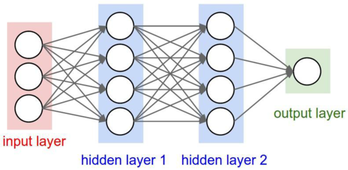
Convolutional Neural Network (CNN) is a kind of feedforward neural network. It has long been one of the core algorithms in the field of image recognition
This is a schematic diagram of roll and neural network mechanism. Let's understand the following parts:
- Input Layer: for us, the input is a picture, but for the computer, the input is a matrix type data, which represents the pixel value of the picture
- Convolution Layer: feature extraction is performed on the input data. Each convolution kernel extracts a feature value from a small area each time. All the feature values are combined to get a feature map. When multiple convolution checks are used for feature extraction, multiple feature maps are obtained. This convolution kernel is called (kernel)
- Activation Function: a function running on the neuron of the artificial neural network, which is responsible for mapping the input of the neuron to the output. The purpose of introducing Activation Function is to increase the nonlinearity of the neural network model
- Pooling Layer: compress images without affecting feature quality to reduce parameters. There are two main types of pooling: MaxPooling and AvePooling. Suppose that the pooled kernel is a 2 * 2 matrix, and MaxPooling is the maximum output value, and AvePooling is the average output value of all data
- Full connected layer (FC for short): it plays the role of "Classifier" in the whole convolutional neural network. If the operations of volume layer, pool layer and activation function layer are to map the original data to the hidden layer feature space, the full connection layer is to map the learned "distributed feature representation" to the sample marker space
- Output Layer: the upstream of the Output Layer in the convolutional neural network is usually the full connection layer, so its structure and working principle are the same as the Output Layer in the traditional feedforward neural network. For image classification, the Output Layer uses the logic function or the softmax function to output the classification label [. In object detection, the Output Layer can be designed as the center coordinate, size and classification of the output object. In image semantic segmentation, the Output Layer directly outputs the classification results of each pixel
After understanding the convolutional neural network, let's look at the convolutional neural network in PyTorch
3. Convolution neural network in PyTorch
3.1 convolution layer: nn.Conv2d()
Its parameters are as follows:
| parameter | Meaning |
| in_channels | The number of channels for the input signal |
| out_channels | The number of output channels after convolution |
| kernel_size | The shape of convolution kernel. For example, kernel_size=(3, 2) represents the convolution kernel of 3X2. If the width and height are the same, it can only be represented by one number |
| stride | Convolution steps per move, default is 1 |
| padding | The number of padding 0 when processing the boundary. The default is 0 (no padding) |
| dilation | Number of sampling intervals, default is 1, no interval sampling |
| groups | The number of packets for input and output channels. When it is not 1, it defaults to 1 (full connection |
| bias | When True, add the offset |
3.2 pool layer: nn.MaxPool2d()
Its parameters are as follows:
| parameter | Meaning |
| kernel_size | Window size at maximum pooling |
| stride | The step size of window movement during the maximum pooling operation. The default value is kernel_size |
| padding | Number of implicit zeros per edge entered |
| dilation | Parameters used to control the step size of elements in the window |
| return_indices | If it is equal to True, return the maximum index while returning the max pooling result, which is very useful in the subsequent Unpooling |
| ceil_mode | If it is equal to True, when calculating the output size, the up rounding will be used instead of the default down rounding |
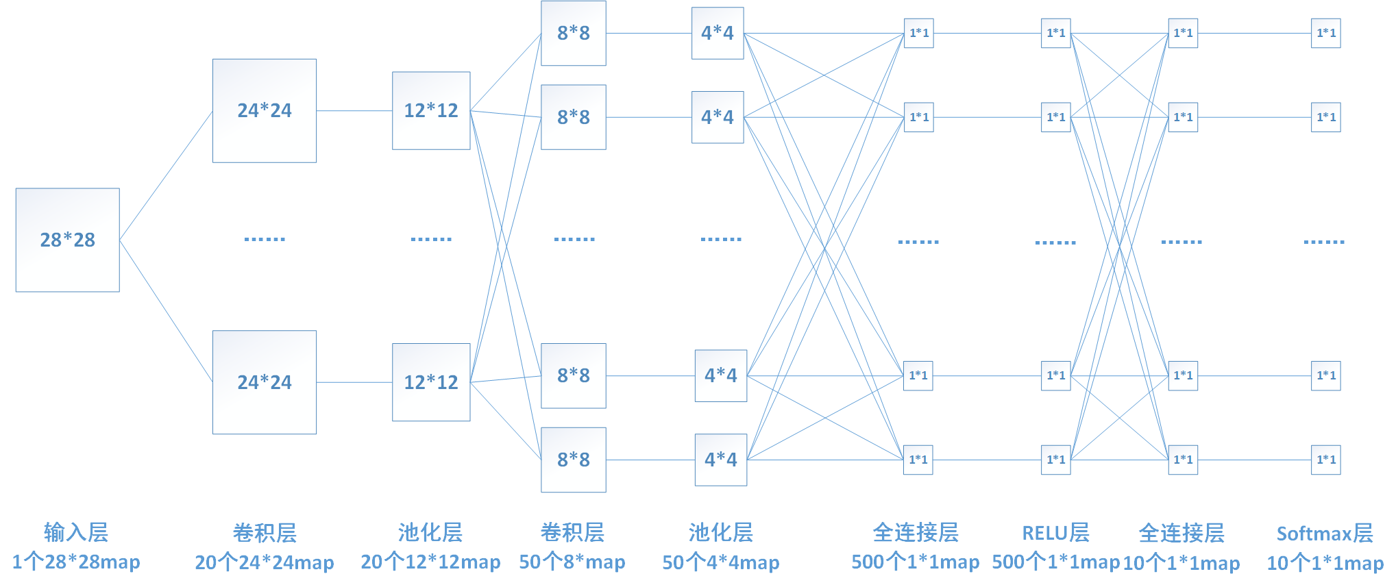
4. MNIST handwritten digit recognition
Now let's use Python to build a convolutional neural network to train and predict handwritten numbers
4.1 import and stock in function
import torch.nn as nn  # The most important module in Python encapsulates the functions related to neural network
import torch.nn.functional as F  # Some common functions are provided, such as softmax
import torch.optim as optim  # The optimization module encapsulates some optimizers for solving the model, such as Adam SGD
from torch.optim import lr_scheduler  # The learning rate adjuster can change the learning rate reasonably in the training process
from torchvision import transforms  # Some interfaces for data transformation are provided in the python visual Library
from torchvision import datasets  # The python visual library provides an interface for loading datasets
4.2 setting super parameters
# Preset network super parameters (so-called super parameters are parameters that can be set artificially

BATCH_SIZE = 64  # Due to the use of batch training method, it is necessary to define the number of samples for each batch of training

EPOCHS = 3  # Total number of training iterations

# Let torch judge whether to use GPU. It is recommended to use GPU environment, because it will be much faster
DEVICE = torch.device("cuda" if torch.cuda.is_available() else "cpu")

learning_rate = 0.001  # Set the initial learning rate
4.3 loading data sets
Here we use the dataloader iterator to load the dataset
# Load training set
train_loader = torch.utils.data.DataLoader(
    datasets.MNIST('data', train=True, download=True,
                   transform=transforms.Compose([
                       transforms.ToTensor(),
                       transforms.Normalize(mean=(0.5,), std=(0.5,))  # Data normalization to normal distribution
                   ])),
    batch_size=BATCH_SIZE, shuffle=True)  # Indicating the batch size and disruption is the need for follow-up training.

test_loader = torch.utils.data.DataLoader(
    datasets.MNIST('data', train=False, transform=transforms.Compose([
        transforms.ToTensor(),
        transforms.Normalize((0.5,), (0.5,))
    ])),
    batch_size=BATCH_SIZE, shuffle=True)
The purpose of the above codes is to:
- Download the mnist training set and test set to the folder data
- Change the data, including changing to the sensor data type, and normalizing the data to the normal distribution to ensure the independent and identical distribution of the training set test set
- The data is stored in batches, and the sequence is disordered for the convenience of subsequent training.
4.4 design CNN
The structure of a simple convolution neural network generally includes:
Convolution layer Conv: extract image features through convolution kernel to get feature map
Pool layer: use convolution check feature map to reduce sampling and size. The maximum pooling layer is the largest pixel in the sliding window, and the average pooling layer is the average pixel result in the sliding window.
Full connection layer: multiple linear model s + activation function eg: ReLU.
This constitutes a basic CNN, but out of a learning mentality, we'd better understand some tricks in the process of in-depth learning and training to improve the generalization ability of the model. Such as:
batch normalization: it is simply to normalize all the output results of the weighted sum of the previous layer in batches (standard normal distribution), then input a linear model, and then connect to the activation function.
DropOut: in the full connection layer, we set the probability randomly to make some weights of this layer 0, which is equivalent to the ineffectiveness of neurons.
# design a model
class ConvNet(nn.Module):
    def __init__(self):
        super(ConvNet, self).__init__()
        # Extract feature layer
        self.features = nn.Sequential(
            # Convolution layer
            # The input image channel is 1, because we use black-and-white image, single channel
            # The output channel is 32 (representing the use of 32 convolution kernels). A convolution kernel generates a single channel characteristic graph
            # The size of convolution kernel_is 3 * 3, and the number of moving pixels represented by stripe is 1
            # padding: 1 means that there are two more pixels in the length and width of the image
            nn.Conv2d(in_channels=1, out_channels=32, kernel_size=3, stride=1, padding=1),# ((28-3+2*1)/1)+1=28  28*28*1  > 28*28*32

            # For batch normalization, the out channels of the next layer are the same size, and the following channel rules must be well matched
            nn.BatchNorm2d(num_features=32),   #28*28*32  > 28*28*32

            # Activation function, inplace=true means direct operation
            nn.ReLU(inplace=True),
            nn.Conv2d(32, 32, kernel_size=3, stride=1, padding=1),   #  ((28-3+2*1)/1)+1=28     28*28*32 > 28*28*32
            nn.BatchNorm2d(32),
            nn.ReLU(inplace=True),

            # Maximum pool layer
            # A sliding window with a kernel size of 2 * 2
            # A stripe of 2 indicates that each sliding distance is 2 pixels
            # After this step, the size of the image becomes 1 / 4, that is, 28 * 28 - '7 * 7
            nn.MaxPool2d(kernel_size=2, stride=2),
            nn.Conv2d(32, 64, kernel_size=3, padding=1),
            nn.BatchNorm2d(64),
            nn.ReLU(inplace=True),
            nn.Conv2d(64, 64, kernel_size=3, padding=1),
            nn.BatchNorm2d(64),
            nn.ReLU(inplace=True),
            nn.MaxPool2d(kernel_size=2, stride=2)
        )
        # Taxonomy
        self.classifier = nn.Sequential(
            # Dropout level
            # p = 0.5 means that there is a possibility of 0.5 for each weight of the layer
            nn.Dropout(p=0.5),
            # Here is the number of channels 64 * image size 7 * 7, and then input to 512 neurons
            nn.Linear(64 * 7 * 7, 512),
            nn.BatchNorm1d(512),
            nn.ReLU(inplace=True),
            nn.Dropout(p=0.5),
            nn.Linear(512, 512),
            nn.BatchNorm1d(512),
            nn.ReLU(inplace=True),
            nn.Dropout(p=0.5),
            nn.Linear(512, 10),
        )
    # Forward transfer function
    def forward(self, x):
        # Through feature extraction layer
        x = self.features(x)
        # The output must be flattened to a one-dimensional vector
        x = x.view(x.size(0), -1)
        x = self.classifier(x)
        return x
4.5 preparation before training
# Initialization model moves network operation to GPU or CPU

ConvModel = ConvNet().to(DEVICE)
# Define cross entropy loss function
criterion = nn.CrossEntropyLoss().to(DEVICE)
# Define model optimizer: input model parameters and define initial learning rate
optimizer = torch.optim.Adam(ConvModel.parameters(), lr=learning_rate)
# Define learning rate scheduler: input the model of packing, define learning rate decay period step_size, gamma is the multiplication factor of decay
exp_lr_scheduler = lr_scheduler.StepLR(optimizer, step_size=6, gamma=0.1)
# Explanation on the official website. If the initial learning rate lr = 0.05, the decay period step_size is 30, and the decay multiplication factor gamma=0.01
# Assuming optimizer uses lr = 0.05 for all groups
# >>> # lr = 0.05     if epoch < 30
# >>> # lr = 0.005    if 30 <= epoch < 60
# >>> # lr = 0.0005   if 60 <= epoch < 90
4.6 training
def train(num_epochs, _model, _device, _train_loader, _optimizer, _lr_scheduler):
    _model.train()  # Set the model to training mode
    _lr_scheduler.step() # Set learning rate scheduler to prepare for update
    for epoch in range(num_epochs):
        # Extract images and tags from iterators
        for i, (images, labels) in enumerate(_train_loader):
            samples = images.to(_device)
            labels = labels.to(_device)
            # At this time, the sample is a batch of pictures. In CNN's input, we need to change it into four dimensions,
            # reshape the first - 1 represents the number of automatically calculated batch pictures n
            # The final result of reshape is n pictures, each picture is 28 * 28 of a single channel, and four-dimensional tensor is obtained
            output = _model(samples.reshape(-1, 1, 28, 28))
            # Calculate loss function value
            loss = criterion(output, labels)
            # Optimizer internal parameter gradient must be 0
            optimizer.zero_grad()
            # Back propagation of loss value
            loss.backward()
            # Update model parameters
            optimizer.step()
            if (i + 1) % 100 == 0:
                print("Epoch:{}/{}, step:{}, loss:{:.4f}".format(epoch + 1, num_epochs, i + 1, loss.item()))
4.7 forecast
def test(_test_loader, _model, _device):
    _model.eval()  # Set the model to enter the prediction mode evaluation
    loss = 0
    correct = 0

    with torch.no_grad():  # If you don't need backward to update the gradient, you need to disable gradient calculation to reduce the waste of memory and computing resources.
        for data, target in _test_loader:
            data, target = data.to(_device), target.to(_device)
            output = ConvModel(data.reshape(-1, 1, 28, 28))
            loss += criterion(output, target).item()  # Add loss value
            pred = output.data.max(1, keepdim=True)[1]  # Find the subscript with the highest probability, which is the output value
            correct += pred.eq(target.data.view_as(pred)).cpu().sum()  # . cpu() is to migrate parameters to the cpu.

    loss /= len(_test_loader.dataset)

    print('\nAverage loss: {:.4f}, Accuracy: {}/{} ({:.3f}%)\n'.format(
        loss, correct, len(_test_loader.dataset),
        100. * correct / len(_test_loader.dataset)))
4.8 operation
for epoch in range(1, EPOCHS + 1):
    train(epoch, ConvModel, DEVICE, train_loader, optimizer, exp_lr_scheduler)
    test(test_loader,ConvModel, DEVICE)
    test(train_loader,ConvModel, DEVICE)
5 Results
pytorch =0.4 run with CPU
Epoch:1/1, step:100, loss:0.1579
Epoch:1/1, step:200, loss:0.0809
Epoch:1/1, step:300, loss:0.0673
Epoch:1/1, step:400, loss:0.1391
Epoch:1/1, step:500, loss:0.0323
Epoch:1/1, step:600, loss:0.0870
Epoch:1/1, step:700, loss:0.0441
Epoch:1/1, step:800, loss:0.0705
Epoch:1/1, step:900, loss:0.0396

Average loss: 0.0006, Accuracy: 9881/10000 (98.000%)

Epoch:1/2, step:100, loss:0.0487
Epoch:1/2, step:200, loss:0.1519
Epoch:1/2, step:300, loss:0.0262
Epoch:1/2, step:400, loss:0.2133
Epoch:1/2, step:500, loss:0.0161
Epoch:1/2, step:600, loss:0.0805
Epoch:1/2, step:700, loss:0.0927
Epoch:1/2, step:800, loss:0.0663
Epoch:1/2, step:900, loss:0.0669
Epoch:2/2, step:100, loss:0.0124
Epoch:2/2, step:200, loss:0.0527
Epoch:2/2, step:300, loss:0.0256
Epoch:2/2, step:400, loss:0.0138
Epoch:2/2, step:500, loss:0.0894
Epoch:2/2, step:600, loss:0.1030
Epoch:2/2, step:700, loss:0.0528
Epoch:2/2, step:800, loss:0.1106
Epoch:2/2, step:900, loss:0.0044

Average loss: 0.0003, Accuracy: 9930/10000 (99.000%)
Epidemic at home, a small project a day come on! Tomorrow we will use visdom to visualize the network!
Reference resources:
https://blog.csdn.net/out_of_memory_error/article/details/81434907

