In-depth learning for beginners (1): The construction of Keras and multi-layer perceptron for beginners
1. Creating environment and installation dependencies
As a Python release, Anaconda contains a large number of science packages and its own environment management tool Conda. Conda and Pip are recommended to build projects.
1.1 Creating a Virtual Environment
Conda is an open source package management system and environment management system for installing multiple versions of packages and their dependencies, and easily switching between them.
Now we will create the environment we need for the first project. We will name it dlwork, use Python version 3.6, open the terminal, and enter the command line "conda create-n environment name python = version number" to create the environment.
(base) jingyudeMacBook-Pro:~ jingyuyan$ conda create -n keras python=3.6
After creating the environment, you need to activate the created environment by "conda activate + environment name":
(base) jingyudeMacBook-Pro:~ jingyuyan$ conda activate dlwork
Or use "source activate + environment name" to activate:
(base) jingyudeMacBook-Pro:~ jingyuyan$ source activate dlwork
1.2 Installation Dependence
Installation of jupyter notebook in the new environment is recommended using the "conda install jupyter" command:
conda install jupyter
After the installation of jupyter notebook, we continue to install some environment dependencies such as TensorFlow, Keras, OpenCV, etc.
The dependency commands to be installed are as follows:
TensorFlow is the backend of keras. In view of the basic tutorial, the version used in this environment is the CPU version. The following chapters will describe how to install and configure the installation of GPU environment training. It is noteworthy that under the CPU version, TensorFlow installed with conda has been using MKL-DNN since version 1.9.0. The speed is the T installed with pip form. Since ensorFlow is eight times higher than that, it is recommended to install TensorFlow using conda install command:
conda install tensorflow
Keras can be used as the top-level Api interface of TensorFlow to simplify the implementation difficulty of many complex algorithms. A more concise code can be used to build and train the neural network. The installation code is as follows:
conda install keras
As a cross-platform computer vision library, OpenCV has very powerful functions in image processing. It is noteworthy that the new version of OpenCV4.x is quite different from the version of 3.x. OpenCV3.4.20 is adopted:
pip install opencv-python==3.4.5.20
Pandas is a tool based on NumPy, which incorporates a large number of libraries and some standard data models, and provides the tools needed to operate large data sets efficiently. The installation method is as follows:
conda install pandas
After installing all the required dependencies, you can use "conda list" to view the currently installed dependencies
conda list
2. Building projects
Create a directory for the current project in the specified disk path. linux or macos can use mkdir command to create a folder directory. Windows can directly use the graphical interface right-click to create a new folder. For example, the directory for our project is project 01:
(dlwork) jingyudeMacBook-Pro:~ jingyuyan$ mkdir project01
After successful creation, in the dlwork environment, enter the project 01 directory and open jupyter notebook:
    cd project01

    jupyter notebook
Create a new ipynb file and enter it

3. MNIST Data Set Downloading and Preprocessing
The data set we adopt is MNIST handwritten digital set. The collector of the data set is Yann LeCun, father of convolutional neural network. MNIST data is composed of thousands of 28 *28 monochrome pictures. It is relatively simple and suitable for in-depth learning of freshmen.
3.1 Import related modules and download data
Import the dependent modules you need to use
import numpy as np
from keras.utils import np_utils
from keras.datasets import mnist
import pandas as pd
import matplotlib.pyplot as plt
Using TensorFlow backend.
When importing keras, "Using TensorFlow backend." indicates that the system automatically uses TensorFlow as the backend of keras.
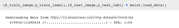
Using mnist.load_data() to download MNIST data sets will take a long time to download first. Please wait patiently for the data sets to be downloaded.
(X_train_image,y_train_label),(X_test_image,y_test_label) = mnist.load_data()
Data sets under Windows will be placed in C: Users XXX. keras datasets mnist. npz
Linux and MacOS systems are placed in ~/.keras/datasets/mnist.npz
If you can't download it or it's too slow for online reasons, you can download mnist.npz directly to the disk provided by this book and place it in the catalog by yourself.
3.2 Data Preprocessing
3.2.1 Reading Data Set Information
After successfully downloading the dataset, you need to re-execute the code to read the dataset. If it does not show that you need to download the dataset, it means that the reading of the dataset is successful.
# Reading Training Set Test Set in Data Set
(X_train_image,y_train_label),(X_test_image,y_test_label) = mnist.load_data()
# View the number of training set test set data in the data set
X_train_image.shape, X_test_image.shape
((60000, 28, 28), (10000, 28, 28))
You can see that the training set and the test set in the above code output dataset have 60 000 and 10 000 single-channel pictures of 28 x 28, respectively.
3.2.2 View images and labels in data sets
In order to understand the direct relationship between images and labels in data sets more conveniently, we write visual scripts to output images and labels.
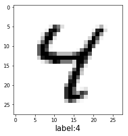
# Define a function that can output pictures and numbers
def show_image(images, labels, idx):
    fig = plt.gcf()
    plt.imshow(images[idx], cmap='binary')
    plt.xlabel('label:'+str(labels[idx]), fontsize = 15)
    plt.show()
show_image(X_train_image, y_train_label, 4)
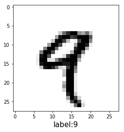
You can see that the code above looks at the image and the corresponding label in the fifth data set of the training set, which are all 9.
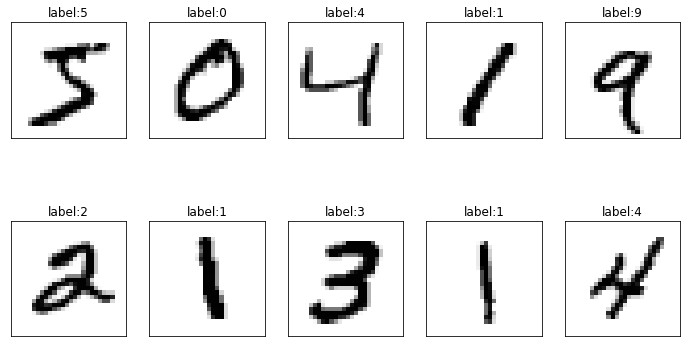
To make it easier to view the data set, we define a function that traverses the overprint graph.
def show_images_set(images,labels,prediction,idx,num=10):
    fig = plt.gcf()
    fig.set_size_inches(12,14)
    for i in range(0,num):
        ax = plt.subplot(4,5,1+i)
        ax.imshow(images[idx],cmap='binary')
        title = "label:"+str(labels[idx])
        if len(prediction)>0:
            title +=",predict="+str(prediction[idx])
        ax.set_title(title,fontsize=12)
        ax.set_xticks([]);ax.set_yticks([])
        idx+=1
    plt.show()
Use show_images_set to display the data of the training set. Prediction is the data set of incoming prediction results, which is temporarily empty here, and idx is the data that needs to be traversed from the first item. By default, num=10 items
show_images_set(images=X_train_image, labels=y_train_label, prediction=[], idx=0)
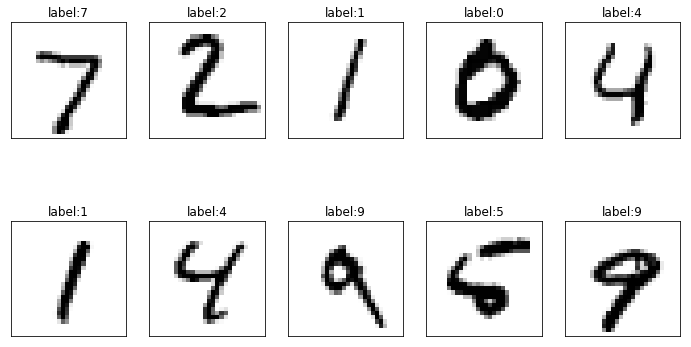
Use show_images_set to display test set data.
show_images_set(images=X_test_image, labels=y_test_label, prediction=[], idx=0)
3.2.3 Data Set Image Preprocessing Operation
Converting an image (28 x 28) from a data set to a one-dimensional vector and then to a data type of Float32
X_Train = X_train_image.reshape(60000, 28*28).astype('float32')
X_Test = X_test_image.reshape(10000, 28*28).astype('float32')
View the converted data output, and see item 5 here.
X_Train[4]
array([  0.,   0.,   0.,   0.,   0.,   0.,   0.,   0.,   0.,   0.,   0.,
         0.,   0.,   0.,   0.,   0.,   0.,   0.,   0.,   0.,   0.,   0.,
         0.,   0.,   0.,   0.,   0.,   0.,   0.,   0.,   0.,   0.,   0.,
         0.,   0.,   0.,   0.,   0.,   0.,   0.,   0.,   0.,   0.,   0.,
         0.,   0.,   0.,   0.,   0.,   0.,   0.,   0.,   0.,   0.,   0.,
         0.,   0.,   0.,   0.,   0.,   0.,   0.,   0.,   0.,   0.,   0.,
         0.,   0.,   0.,   0.,   0.,   0.,   0.,   0.,   0.,   0.,   0.,
         0.,   0.,   0.,   0.,   0.,   0.,   0.,   0.,   0.,   0.,   0.,
         0.,   0.,   0.,   0.,   0.,   0.,   0.,   0.,   0.,   0.,   0.,
         0.,   0.,   0.,   0.,   0.,   0.,   0.,   0.,   0.,   0.,   0.,
         0.,   0.,   0.,   0.,   0.,   0.,   0.,   0.,   0.,   0.,   0.,
         0.,   0.,   0.,   0.,   0.,   0.,   0.,   0.,   0.,   0.,   0.,
         0.,   0.,   0.,   0.,   0.,   0.,   0.,   0.,   0.,   0.,   0.,
         0.,   0.,   0.,   0.,   0.,   0.,   0.,   0.,   0.,   0.,   0.,
         0.,   0.,   0.,   0.,   0.,   0.,   0.,   0.,   0.,   0.,   0.,
         0.,   0.,   0.,   0.,   0.,   0.,   0.,   0.,   0.,   0.,   0.,
         0.,   0.,   0.,   0.,   0.,   0.,   0.,   0.,   0.,   0.,   0.,
         0.,   0.,   0.,   0.,   0.,   0.,   0.,   0.,   0.,   0.,   0.,
         0.,   0.,   0.,   0.,   0.,   0.,   0.,   0.,   0.,   0.,  55.,
       148., 210., 253., 253., 113.,  87., 148.,  55.,   0.,   0.,   0.,
         0.,   0.,   0.,   0.,   0.,   0.,   0.,   0.,   0.,   0.,   0.,
         0.,   0.,   0.,   0.,  87., 232., 252., 253., 189., 210., 252.,
       252., 253., 168.,   0.,   0.,   0.,   0.,   0.,   0.,   0.,   0.,
         0.,   0.,   0.,   0.,   0.,   0.,   0.,   0.,   4.,  57., 242.,
       252., 190.,  65.,   5.,  12., 182., 252., 253., 116.,   0.,   0.,
         0.,   0.,   0.,   0.,   0.,   0.,   0.,   0.,   0.,   0.,   0.,
         0.,   0.,   0.,  96., 252., 252., 183.,  14.,   0.,   0.,  92.,
       252., 252., 225.,  21.,   0.,   0.,   0.,   0.,   0.,   0.,   0.,
         0.,   0.,   0.,   0.,   0.,   0.,   0.,   0., 132., 253., 252.,
       146.,  14.,   0.,   0.,   0., 215., 252., 252.,  79.,   0.,   0.,
         0.,   0.,   0.,   0.,   0.,   0.,   0.,   0.,   0.,   0.,   0.,
         0.,   0., 126., 253., 247., 176.,   9.,   0.,   0.,   8.,  78.,
       245., 253., 129.,   0.,   0.,   0.,   0.,   0.,   0.,   0.,   0.,
         0.,   0.,   0.,   0.,   0.,   0.,   0.,  16., 232., 252., 176.,
         0.,   0.,   0.,  36., 201., 252., 252., 169.,  11.,   0.,   0.,
         0.,   0.,   0.,   0.,   0.,   0.,   0.,   0.,   0.,   0.,   0.,
         0.,   0.,  22., 252., 252.,  30.,  22., 119., 197., 241., 253.,
       252., 251.,  77.,   0.,   0.,   0.,   0.,   0.,   0.,   0.,   0.,
         0.,   0.,   0.,   0.,   0.,   0.,   0.,   0.,  16., 231., 252.,
       253., 252., 252., 252., 226., 227., 252., 231.,   0.,   0.,   0.,
         0.,   0.,   0.,   0.,   0.,   0.,   0.,   0.,   0.,   0.,   0.,
         0.,   0.,   0.,   0.,  55., 235., 253., 217., 138.,  42.,  24.,
       192., 252., 143.,   0.,   0.,   0.,   0.,   0.,   0.,   0.,   0.,
         0.,   0.,   0.,   0.,   0.,   0.,   0.,   0.,   0.,   0.,   0.,
         0.,   0.,   0.,   0.,   0.,  62., 255., 253., 109.,   0.,   0.,
         0.,   0.,   0.,   0.,   0.,   0.,   0.,   0.,   0.,   0.,   0.,
         0.,   0.,   0.,   0.,   0.,   0.,   0.,   0.,   0.,   0.,   0.,
        71., 253., 252.,  21.,   0.,   0.,   0.,   0.,   0.,   0.,   0.,
         0.,   0.,   0.,   0.,   0.,   0.,   0.,   0.,   0.,   0.,   0.,
         0.,   0.,   0.,   0.,   0.,   0.,   0., 253., 252.,  21.,   0.,
         0.,   0.,   0.,   0.,   0.,   0.,   0.,   0.,   0.,   0.,   0.,
         0.,   0.,   0.,   0.,   0.,   0.,   0.,   0.,   0.,   0.,   0.,
         0.,  71., 253., 252.,  21.,   0.,   0.,   0.,   0.,   0.,   0.,
         0.,   0.,   0.,   0.,   0.,   0.,   0.,   0.,   0.,   0.,   0.,
         0.,   0.,   0.,   0.,   0.,   0.,   0., 106., 253., 252.,  21.,
         0.,   0.,   0.,   0.,   0.,   0.,   0.,   0.,   0.,   0.,   0.,
         0.,   0.,   0.,   0.,   0.,   0.,   0.,   0.,   0.,   0.,   0.,
         0.,   0.,  45., 255., 253.,  21.,   0.,   0.,   0.,   0.,   0.,
         0.,   0.,   0.,   0.,   0.,   0.,   0.,   0.,   0.,   0.,   0.,
         0.,   0.,   0.,   0.,   0.,   0.,   0.,   0.,   0., 218., 252.,
        56.,   0.,   0.,   0.,   0.,   0.,   0.,   0.,   0.,   0.,   0.,
         0.,   0.,   0.,   0.,   0.,   0.,   0.,   0.,   0.,   0.,   0.,
         0.,   0.,   0.,   0.,  96., 252., 189.,  42.,   0.,   0.,   0.,
         0.,   0.,   0.,   0.,   0.,   0.,   0.,   0.,   0.,   0.,   0.,
         0.,   0.,   0.,   0.,   0.,   0.,   0.,   0.,   0.,   0.,  14.,
       184., 252., 170.,  11.,   0.,   0.,   0.,   0.,   0.,   0.,   0.,
         0.,   0.,   0.,   0.,   0.,   0.,   0.,   0.,   0.,   0.,   0.,
         0.,   0.,   0.,   0.,   0.,   0.,  14., 147., 252.,  42.,   0.,
         0.,   0.,   0.,   0.,   0.,   0.,   0.,   0.,   0.,   0.,   0.,
         0.,   0.,   0.,   0.,   0.,   0.,   0.,   0.,   0.,   0.,   0.,
         0.,   0.,   0.,   0.,   0.,   0.,   0.,   0.,   0.,   0.,   0.,
         0.,   0.,   0.], dtype=float32)
Most of the vectors output above a clear hairstyle are 0, representing the colorless area, and the number between 0 and 255 is the degree of color of each gray point represented in the image.
After transforming the image, we normalize the image, that is, mapping the number from 0 to 255 to the number between 0 and 1, which can refer to the accuracy of model training.
X_Train_normalize = X_Train / 255
X_Test_normalize = X_Test / 255
By looking at the normalization results, we can see that after normalization and output data, all the previous 0-255 numbers mapped to the number between 0 and 1.
X_Train_normalize[4]
array([0. , 0. , 0. , 0. , 0. ,
0. , 0. , 0. , 0. , 0. ,
0. , 0. , 0. , 0. , 0. ,
0. , 0. , 0. , 0. , 0. ,
0. , 0. , 0. , 0. , 0. ,
0. , 0. , 0. , 0. , 0. ,
0. , 0. , 0. , 0. , 0. ,
0. , 0. , 0. , 0. , 0. ,
0. , 0. , 0. , 0. , 0. ,
0. , 0. , 0. , 0. , 0. ,
0. , 0. , 0. , 0. , 0. ,
0. , 0. , 0. , 0. , 0. ,
0. , 0. , 0. , 0. , 0. ,
0. , 0. , 0. , 0. , 0. ,
0. , 0. , 0. , 0. , 0. ,
0. , 0. , 0. , 0. , 0. ,
0. , 0. , 0. , 0. , 0. ,
0. , 0. , 0. , 0. , 0. ,
0. , 0. , 0. , 0. , 0. ,
0. , 0. , 0. , 0. , 0. ,
0. , 0. , 0. , 0. , 0. ,
0. , 0. , 0. , 0. , 0. ,
0. , 0. , 0. , 0. , 0. ,
0. , 0. , 0. , 0. , 0. ,
0. , 0. , 0. , 0. , 0. ,
0. , 0. , 0. , 0. , 0. ,
0. , 0. , 0. , 0. , 0. ,
0. , 0. , 0. , 0. , 0. ,
0. , 0. , 0. , 0. , 0. ,
0. , 0. , 0. , 0. , 0. ,
0. , 0. , 0. , 0. , 0. ,
0. , 0. , 0. , 0. , 0. ,
0. , 0. , 0. , 0. , 0. ,
0. , 0. , 0. , 0. , 0. ,
0. , 0. , 0. , 0. , 0. ,
0. , 0. , 0. , 0. , 0. ,
0. , 0. , 0. , 0. , 0. ,
0. , 0. , 0. , 0. , 0. ,
0. , 0. , 0. , 0. , 0. ,
0. , 0. , 0. , 0. , 0. ,
0. , 0. , 0. , 0. , 0. ,
0. , 0. , 0. , 0.21568628, 0.5803922 ,
0.8235294 , 0.99215686, 0.99215686, 0.44313726, 0.34117648,
0.5803922 , 0.21568628, 0. , 0. , 0. ,
0. , 0. , 0. , 0. , 0. ,
0. , 0. , 0. , 0. , 0. ,
0. , 0. , 0. , 0. , 0. ,
0.34117648, 0.9098039 , 0.9882353 , 0.99215686, 0.7411765 ,
0.8235294 , 0.9882353 , 0.9882353 , 0.99215686, 0.65882355,
0. , 0. , 0. , 0. , 0. ,
0. , 0. , 0. , 0. , 0. ,
0. , 0. , 0. , 0. , 0. ,
0. , 0.01568628, 0.22352941, 0.9490196 , 0.9882353 ,
0.74509805, 0.25490198, 0.01960784, 0.04705882, 0.7137255 ,
0.9882353 , 0.99215686, 0.45490196, 0. , 0. ,
0. , 0. , 0. , 0. , 0. ,
0. , 0. , 0. , 0. , 0. ,
0. , 0. , 0. , 0. , 0.3764706 ,
0.9882353 , 0.9882353 , 0.7176471 , 0.05490196, 0. ,
0. , 0.36078432, 0.9882353 , 0.9882353 , 0.88235295,
0.08235294, 0. , 0. , 0. , 0. ,
0. , 0. , 0. , 0. , 0. ,
0. , 0. , 0. , 0. , 0. ,
0. , 0.5176471 , 0.99215686, 0.9882353 , 0.57254905,
0.05490196, 0. , 0. , 0. , 0.84313726,
0.9882353 , 0.9882353 , 0.30980393, 0. , 0. ,
0. , 0. , 0. , 0. , 0. ,
0. , 0. , 0. , 0. , 0. ,
0. , 0. , 0. , 0.49411765, 0.99215686,
0.96862745, 0.6901961 , 0.03529412, 0. , 0. ,
0.03137255, 0.30588236, 0.9607843 , 0.99215686, 0.5058824 ,
0. , 0. , 0. , 0. , 0. ,
0. , 0. , 0. , 0. , 0. ,
0. , 0. , 0. , 0. , 0. ,
0.0627451 , 0.9098039 , 0.9882353 , 0.6901961 , 0. ,
0. , 0. , 0.14117648, 0.7882353 , 0.9882353 ,
0.9882353 , 0.6627451 , 0.04313726, 0. , 0. ,
0. , 0. , 0. , 0. , 0. ,
0. , 0. , 0. , 0. , 0. ,
0. , 0. , 0. , 0.08627451, 0.9882353 ,
0.9882353 , 0.11764706, 0.08627451, 0.46666667, 0.77254903,
0.94509804, 0.99215686, 0.9882353 , 0.9843137 , 0.3019608 ,
0. , 0. , 0. , 0. , 0. ,
0. , 0. , 0. , 0. , 0. ,
0. , 0. , 0. , 0. , 0. ,
0. , 0.0627451 , 0.90588236, 0.9882353 , 0.99215686,
0.9882353 , 0.9882353 , 0.9882353 , 0.8862745 , 0.8901961 ,
0.9882353 , 0.90588236, 0. , 0. , 0. ,
0. , 0. , 0. , 0. , 0. ,
0. , 0. , 0. , 0. , 0. ,
0. , 0. , 0. , 0. , 0. ,
0.21568628, 0.92156863, 0.99215686, 0.8509804 , 0.5411765 ,
0.16470589, 0.09411765, 0.7529412 , 0.9882353 , 0.56078434,
0. , 0. , 0. , 0. , 0. ,
0. , 0. , 0. , 0. , 0. ,
0. , 0. , 0. , 0. , 0. ,
0. , 0. , 0. , 0. , 0. ,
0. , 0. , 0. , 0. , 0.24313726,
1. , 0.99215686, 0.42745098, 0. , 0. ,
0. , 0. , 0. , 0. , 0. ,
0. , 0. , 0. , 0. , 0. ,
0. , 0. , 0. , 0. , 0. ,
0. , 0. , 0. , 0. , 0. ,
0. , 0. , 0.2784314 , 0.99215686, 0.9882353 ,
0.08235294, 0. , 0. , 0. , 0. ,
0. , 0. , 0. , 0. , 0. ,
0. , 0. , 0. , 0. , 0. ,
0. , 0. , 0. , 0. , 0. ,
0. , 0. , 0. , 0. , 0. ,
0. , 0.99215686, 0.9882353 , 0.08235294, 0. ,
0. , 0. , 0. , 0. , 0. ,
0. , 0. , 0. , 0. , 0. ,
0. , 0. , 0. , 0. , 0. ,
0. , 0. , 0. , 0. , 0. ,
0. , 0. , 0. , 0.2784314 , 0.99215686,
0.9882353 , 0.08235294, 0. , 0. , 0. ,
0. , 0. , 0. , 0. , 0. ,
0. , 0. , 0. , 0. , 0. ,
0. , 0. , 0. , 0. , 0. ,
0. , 0. , 0. , 0. , 0. ,
0. , 0.41568628, 0.99215686, 0.9882353 , 0.08235294,
0. , 0. , 0. , 0. , 0. ,
0. , 0. , 0. , 0. , 0. ,
0. , 0. , 0. , 0. , 0. ,
0. , 0. , 0. , 0. , 0. ,
0. , 0. , 0. , 0. , 0.1764706 ,
1. , 0.99215686, 0.08235294, 0. , 0. ,
0. , 0. , 0. , 0. , 0. ,
0. , 0. , 0. , 0. , 0. ,
0. , 0. , 0. , 0. , 0. ,
0. , 0. , 0. , 0. , 0. ,
0. , 0. , 0. , 0.85490197, 0.9882353 ,
0.21960784, 0. , 0. , 0. , 0. ,
0. , 0. , 0. , 0. , 0. ,
0. , 0. , 0. , 0. , 0. ,
0. , 0. , 0. , 0. , 0. ,
0. , 0. , 0. , 0. , 0. ,
0. , 0.3764706 , 0.9882353 , 0.7411765 , 0.16470589,
0. , 0. , 0. , 0. , 0. ,
0. , 0. , 0. , 0. , 0. ,
0. , 0. , 0. , 0. , 0. ,
0. , 0. , 0. , 0. , 0. ,
0. , 0. , 0. , 0. , 0.05490196,
0.72156864, 0.9882353 , 0.6666667 , 0.04313726, 0. ,
0. , 0. , 0. , 0. , 0. ,
0. , 0. , 0. , 0. , 0. ,
0. , 0. , 0. , 0. , 0. ,
0. , 0. , 0. , 0. , 0. ,
0. , 0. , 0. , 0.05490196, 0.5764706 ,
0.9882353 , 0.16470589, 0. , 0. , 0. ,
0. , 0. , 0. , 0. , 0. ,
0. , 0. , 0. , 0. , 0. ,
0. , 0. , 0. , 0. , 0. ,
0. , 0. , 0. , 0. , 0. ,
0. , 0. , 0. , 0. , 0. ,
0. , 0. , 0. , 0. , 0. ,
0. , 0. , 0. , 0. ], dtype=float32)
3.2.3 Data Set Image Preprocessing Operation
The label label field is originally a number of 0-9. It must be converted to 10 combinations of 0 or 1 by One-Hot Endcoding (one-bit effective coding), which corresponds to 10 results of the final output layer of the neural network.
y_TrainOneHot = np_utils.to_categorical(y_train_label)
y_TestOneHot = np_utils.to_categorical(y_test_label)
After transformation, we extract labels from the data set for comparison.
y_train_label[:3]
array([5, 0, 4], dtype=uint8)
y_TrainOneHot[:3]
array([[0., 0., 0., 0., 0., 1., 0., 0., 0., 0.],
       [1., 0., 0., 0., 0., 0., 0., 0., 0., 0.],
       [0., 0., 0., 0., 1., 0., 0., 0., 0., 0.]], dtype=float32)
For example, the label number 5 of the first item has been converted to 00000010000.
3.3 First attempt to build multi-layer perceptron for training
3.3.1 Modeling
Firstly, the simplest model is built, which has only input layer and output layer. The parameters of input layer are 28*28=784, and output layer is 10, which corresponds to 10 numbers of numbers.
from keras.models import Sequential
from keras.layers import Dense,Dropout,Flatten,Conv2D,MaxPooling2D,Activation
# Setting model parameters
CLASSES_NB = 10
INPUT_SHAPE = 28 * 28
# Establishment of Sequential Model
model = Sequential()
# Add a Dense layer with input directly as
model.add(Dense(units=CLASSES_NB,
               input_dim=INPUT_SHAPE,))

# Define the output layer and use softmax to activate and convert the results of 10 numbers from 0 to 9 in the form of probability
model.add(Activation('softmax'))
WARNING:tensorflow:From /Users/jingyuyan/anaconda3/envs/dlwork/lib/python3.6/site-packages/tensorflow/python/framework/op_def_library.py:263: colocate_with (from tensorflow.python.framework.ops) is deprecated and will be removed in a future version.
Instructions for updating:
Colocations handled automatically by placer.
Once the model is built, you can view the summary of the model using summary().
model.summary()
_________________________________________________________________
Layer (type)                 Output Shape              Param #
=================================================================
dense_1 (Dense)              (None, 10)                7850
_________________________________________________________________
activation_1 (Activation)    (None, 10)                0
=================================================================
Total params: 7,850
Trainable params: 7,850
Non-trainable params: 0
_________________________________________________________________
3.3.2 Neural Network Training
The multi-layer perceptron model has been established. We can use directional propagation to train the model. The keras training needs to use compile to set training parameters for the model:
- Loss: Loss function is trained with cross_entropy loss function
- Optimizer: using adam optimizer to optimize gradient descent algorithm can accelerate the convergence speed of neural network
- metrics: the evaluation method is set here as the accuracy of the quasi-removal rate
# Setting up training parameters
model.compile(loss='categorical_crossentropy',optimizer='adam',metrics=['accuracy'])
After the training parameters are established, the training begins. Some parameters in the training process need to be configured before training:
# Validation Set Partition Ratio
VALIDATION_SPLIT = 0.2
# Training cycle
EPOCH = 10
# Single batch data volume
BATCH_SIZE = 128
# Training LOG Printing Form
VERBOSE = 2
- epochs: set the training cycle to 10 rounds
- batch_size: Set the data for 128 items in each batch
- validation_split: Validation set is used to divide part of the model into several parts for testing in each round of training. Setting the ratio of verification set to 0.2 indicates that the training data and validation data are divided into 8:2 formats, and the training data are 60,000 items, so the validation set is 12,000 items.
# Input data, start training
# verbose is a training process for representing display printing
train_history = model.fit(
        x=X_Train_normalize,
        y=y_TrainOneHot,
        epochs=EPOCH,
        batch_size=BATCH_SIZE,
        verbose=VERBOSE,
        validation_split=VALIDATION_SPLIT)
WARNING:tensorflow:From /Users/jingyuyan/anaconda3/envs/dlwork/lib/python3.6/site-packages/tensorflow/python/ops/math_ops.py:3066: to_int32 (from tensorflow.python.ops.math_ops) is deprecated and will be removed in a future version.
Instructions for updating:
Use tf.cast instead.
Train on 48000 samples, validate on 12000 samples
Epoch 1/10
 - 1s - loss: 0.7762 - acc: 0.8076 - val_loss: 0.4124 - val_acc: 0.8963
Epoch 2/10
 - 1s - loss: 0.3929 - acc: 0.8955 - val_loss: 0.3348 - val_acc: 0.9091
Epoch 3/10
 - 0s - loss: 0.3402 - acc: 0.9076 - val_loss: 0.3087 - val_acc: 0.9167
Epoch 4/10
 - 0s - loss: 0.3154 - acc: 0.9132 - val_loss: 0.2947 - val_acc: 0.9207
Epoch 5/10
 - 1s - loss: 0.3014 - acc: 0.9160 - val_loss: 0.2847 - val_acc: 0.9212
Epoch 6/10
 - 1s - loss: 0.2913 - acc: 0.9191 - val_loss: 0.2803 - val_acc: 0.9212
Epoch 7/10
 - 1s - loss: 0.2841 - acc: 0.9205 - val_loss: 0.2742 - val_acc: 0.9249
Epoch 8/10
 - 1s - loss: 0.2784 - acc: 0.9222 - val_loss: 0.2714 - val_acc: 0.9255
Epoch 9/10
 - 1s - loss: 0.2738 - acc: 0.9231 - val_loss: 0.2688 - val_acc: 0.9255
Epoch 10/10
 - 1s - loss: 0.2702 - acc: 0.9249 - val_loss: 0.2660 - val_acc: 0.9278
From the logs printed above, it can be seen that after 10 rounds of training, loss gradually decreases and the accuracy is constantly improving.
Define a function, plot the data in the training process, and present it as a chart.
def show_train_history(train_history,train,validation):
    plt.plot(train_history.history[train])
    plt.plot(train_history.history[validation])
    plt.title('Train histoty')
    plt.ylabel(train)
    plt.xlabel('Epoch')
    plt.legend(['train','validation',],loc = 'upper left')
    plt.show()
We import the training results and plot the accuracy of the training process.
show_train_history(train_history,'acc','val_acc')
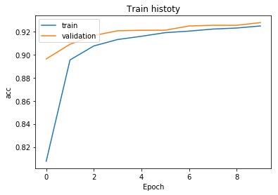
Accuracy (acc) is the blue line obtained from the graph, which is constantly raised in every round of training.
Continue to use the rendering function to plot the error rate image:
show_train_history(train_history,'loss','val_loss')
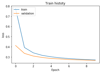
The blue line from the figure is the error rate (loss), which is constantly decreasing in each round of training.
The training log shows that the accuracy of the model is only about 0.92. In the next section, hidden layer neural network will be added to improve the accuracy of the model.
3.4 Improving Hidden Layer Model
3.4.1 Modeling
From now on, a multi-layer perceptron model will be built step by step. There are 784 neurons in the input layer, 256 in the hidden layer and 10 in the output layer, which correspond to the numerical results between 10 and 9, respectively.
CLASSES_NB = 10
INPUT_SHAPE = 28 * 28
UNITS = 256
Rebuild the model, add a hidden layer, deepen and thicken the depth and width of the model.
# Establishment of Sequential Model
model = Sequential()
# Adding a Dense, Deense features both upper and lower network connections
# The Dense layer contains the input layer and the hidden layer.
model.add(Dense(units=UNITS,
               input_dim=INPUT_SHAPE,
               kernel_initializer='normal',
               activation='relu'))

# Define the output layer and use softmax to activate and convert the results of 10 numbers from 0 to 9 in the form of probability
model.add(Dense(CLASSES_NB, activation='softmax'))
# Output model summary after building
model.summary()
_________________________________________________________________
Layer (type)                 Output Shape              Param #
=================================================================
dense_2 (Dense)              (None, 256)               200960
_________________________________________________________________
dense_3 (Dense)              (None, 10)                2570
=================================================================
Total params: 203,530
Trainable params: 203,530
Non-trainable params: 0
_________________________________________________________________
- Hidden layer: 256 neurons
- Output layer: 10 neurons
- dense_1 parameter: 784 x 256 + 256 = 200,960
- dense_2 parameter: 256 x 10 + 10 = 2570
- Total training parameters: 200960 + 2570 = 203,530
3.4.2 Neural Network Training
The multi-layer perceptron model has been established. We can use directional propagation to train the model. The keras training needs to use compile to set training parameters for the model:
# Validation Set Partition Ratio
VALIDATION_SPLIT = 0.2
# Increase training cycle to 20 rounds
EPOCH = 15
# Single batch data volume increased to 300
BATCH_SIZE = 300
# Training LOG Printing Form
VERBOSE = 2
# Setting up training parameters
model.compile(loss='categorical_crossentropy',optimizer='adam',metrics=['accuracy'])
Increase the number of training rounds and batches appropriately
# Input data, start training
# verbose is a training process for representing display printing
train_history = model.fit(
        x=X_Train_normalize,
        y=y_TrainOneHot,
        epochs=EPOCH,
        batch_size=BATCH_SIZE,
        verbose=VERBOSE,
        validation_split=VALIDATION_SPLIT)
Train on 48000 samples, validate on 12000 samples
Epoch 1/15
 - 2s - loss: 0.4466 - acc: 0.8794 - val_loss: 0.2219 - val_acc: 0.9395
Epoch 2/15
 - 1s - loss: 0.1926 - acc: 0.9462 - val_loss: 0.1618 - val_acc: 0.9553
Epoch 3/15
 - 1s - loss: 0.1383 - acc: 0.9612 - val_loss: 0.1339 - val_acc: 0.9625
Epoch 4/15
 - 1s - loss: 0.1092 - acc: 0.9700 - val_loss: 0.1181 - val_acc: 0.9664
Epoch 5/15
 - 1s - loss: 0.0878 - acc: 0.9756 - val_loss: 0.1065 - val_acc: 0.9684
Epoch 6/15
 - 1s - loss: 0.0730 - acc: 0.9793 - val_loss: 0.0961 - val_acc: 0.9716
Epoch 7/15
 - 1s - loss: 0.0614 - acc: 0.9829 - val_loss: 0.0928 - val_acc: 0.9718
Epoch 8/15
 - 1s - loss: 0.0525 - acc: 0.9860 - val_loss: 0.0895 - val_acc: 0.9739
Epoch 9/15
 - 1s - loss: 0.0439 - acc: 0.9885 - val_loss: 0.0861 - val_acc: 0.9744
Epoch 10/15
 - 1s - loss: 0.0378 - acc: 0.9906 - val_loss: 0.0837 - val_acc: 0.9755
Epoch 11/15
 - 1s - loss: 0.0326 - acc: 0.9921 - val_loss: 0.0816 - val_acc: 0.9749
Epoch 12/15
 - 1s - loss: 0.0275 - acc: 0.9934 - val_loss: 0.0789 - val_acc: 0.9765
Epoch 13/15
 - 1s - loss: 0.0233 - acc: 0.9951 - val_loss: 0.0809 - val_acc: 0.9754
Epoch 14/15
 - 1s - loss: 0.0198 - acc: 0.9963 - val_loss: 0.0800 - val_acc: 0.9758
Epoch 15/15
 - 1s - loss: 0.0174 - acc: 0.9967 - val_loss: 0.0793 - val_acc: 0.9759
It can be seen from the log that the accuracy of the model increases and the loss decreases after the hidden layer is introduced, compared with the previous network with only input layer and output layer.
Using the show_train_history function defined in the previous section, the quasi-removal rate and the loss rate of training are plotted respectively.
show_train_history(train_history,'acc','val_acc')
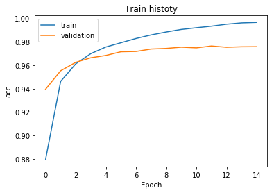
Accuracy (acc) is the blue line that can be obtained with pictures in every round of training, but the validation set accuracy (val_acc) is lower than the accuracy in the later stage of training.
show_train_history(train_history,'loss','val_loss')
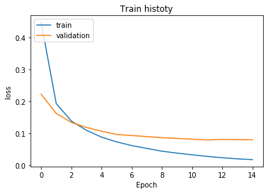
The blue line error rate (loss) obtained from the graph is constantly decreasing in each round of training, while the validation set error rate (val_loss) is higher than the accuracy rate in the later stage of training.
Why is the accuracy rate lower and the error rate higher at the later stage of training? This involves the phenomenon of fitting. Later chapters will elaborate.
3.5 Evaluation of training results
3.5.1 Use Test Set to Evaluate Model Accuracy
Now you need to use the test set data that you loaded before. There are 10,000 pieces of test set data. Because the test set data is not involved in the training of the model, it is usually used to evaluate the accuracy of the model after the model training.
Define a scores to store all the evaluation results, and use the evaluate function to pass the test set pictures and labels into the model for evaluation testing.
scores = model.evaluate(X_Test_normalize, y_TestOneHot)
10000/10000 [==============================] - 0s 24us/step
After the test and prediction are completed, the prediction results are printed out. First, the loss and accuracy of the model are printed out.
print('loss: ',scores[0])
print('accuracy: ',scores[1])
loss:  0.07091819015247747
accuracy:  0.9782
After introducing the hidden layer into the multi-layer perceptron, the prediction accuracy of the training model under the test set can reach 0.97.
3.5.2 Use the model to predict the test set
The test set is passed into the model for prediction, where we try to observe the differences using predicts and predict_classes, respectively.
result = model.predict(X_Test)
result_class = model.predict_classes(X_Test)
Output the real and predicted results of the fifth item of the forecast data separately
# Use the previously defined function for displaying pictures
show_image(X_test_image, y_test_label, 6)
You can see that the image and label for item 7 are all 4.
result[6]
array([0., 0., 0., 0., 1., 0., 0., 0., 0., 0.], dtype=float32)
Using predictive function to predict the output is a vector, that is, the one-hot format of tag processing in the previous section.
result_class[6]
4
As you can see, the predicted results using predict_classes output tag 4 directly, indicating that the result is the fifth classification.
So in order to view the predicted results conveniently, we use the form of predicted_classes predicted results.
Using the functions defined in the preceding section, we can see the predicted and real results of multiple data, and take the following 10 data from item 248 to see.
# Previously, the third parameter was empty when looking at the data. Now there is predicted data. It needs to be passed in to make an intuitive comparison.
show_images_set(X_test_image,y_test_label,result_class,idx=247)
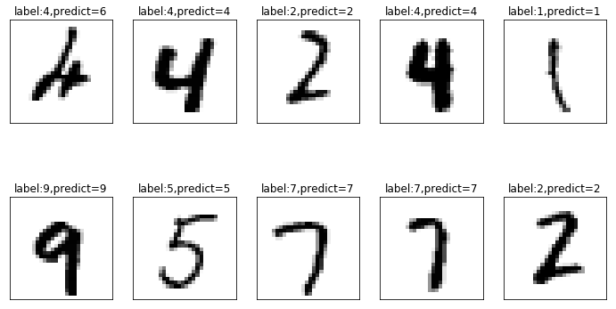
It can be seen that the first item of the result of the above figure has a prediction error. The original value should be 4, but it is mistaken for 6 by the neural network. Because this handwriting is sloppy, it is unavoidable to recognize errors.
3.5.3 Establishment of Error Matrix
In the previous section, we found that in the prediction process, the model will have errors. For example, in the previous section, we found that scribbled handwritten number 4 to model prediction result 6, with such a problem, if we need to find other similar cases, observe which numbers will have larger errors, then we need to establish error matrix, also known as confusion matrix, to display the error map. .
Using the cross tab function of pandas, the label of test set and the label of predicted result can be transferred into the function to establish the error matrix.
# Using pandas Library
import pandas as pd
pd.crosstab(y_test_label, result_class, rownames=['label'], colnames=['predict'])
| predict | 0 | 1 | 2 | 3 | 4 | 5 | 6 | 7 | 8 | 9 |
|---|---|---|---|---|---|---|---|---|---|---|
| label | ||||||||||
| 0 | 971 | 0 | 2 | 2 | 2 | 0 | 1 | 1 | 1 | 0 |
| 1 | 0 | 1127 | 4 | 0 | 0 | 1 | 1 | 0 | 2 | 0 |
| 2 | 4 | 1 | 1012 | 2 | 2 | 1 | 2 | 5 | 3 | 0 |
| 3 | 1 | 1 | 3 | 996 | 0 | 3 | 0 | 3 | 2 | 1 |
| 4 | 1 | 0 | 4 | 0 | 957 | 0 | 5 | 2 | 0 | 13 |
| 5 | 2 | 0 | 0 | 12 | 1 | 866 | 4 | 1 | 4 | 2 |
| 6 | 6 | 3 | 2 | 1 | 3 | 4 | 937 | 1 | 1 | 0 |
| 7 | 0 | 4 | 10 | 2 | 1 | 0 | 0 | 1005 | 0 | 6 |
| 8 | 3 | 0 | 11 | 14 | 2 | 8 | 1 | 4 | 929 | 2 |
| 9 | 5 | 5 | 0 | 9 | 6 | 2 | 0 | 4 | 1 | 977 |
Looking at the error matrix carefully, we can see that the confusion times of 3 and 5 are the highest, followed by 9 and 4.
To make it easier for us to see what kind of data confuses us, we use pandas to create a DataFrame to see the details of the confused data.
# Create DataFrame
dic = {'label':y_test_label, 'predict':result_class}
df = pd.DataFrame(dic)
View all predicted results and the true values of data items
# T is to transpose the matrix for easy viewing of data.
df.T
| 0 | 1 | 2 | 3 | 4 | 5 | 6 | 7 | 8 | 9 | ... | 9990 | 9991 | 9992 | 9993 | 9994 | 9995 | 9996 | 9997 | 9998 | 9999 | |
|---|---|---|---|---|---|---|---|---|---|---|---|---|---|---|---|---|---|---|---|---|---|
| label | 7 | 2 | 1 | 0 | 4 | 1 | 4 | 9 | 5 | 9 | ... | 7 | 8 | 9 | 0 | 1 | 2 | 3 | 4 | 5 | 6 |
| predict | 7 | 2 | 1 | 0 | 4 | 1 | 4 | 9 | 5 | 9 | ... | 7 | 8 | 9 | 0 | 1 | 2 | 3 | 4 | 5 | 6 |
2 rows × 10000 columns
Look at the confused data items 5 and 3. Here we choose to look at the data marked 1670 to see the picture.
df[(df.label==5)&(df.predict==3)].T
| 340 | 1003 | 1393 | 1670 | 2035 | 2597 | 2810 | 4360 | 5937 | 5972 | 5982 | 9422 | |
|---|---|---|---|---|---|---|---|---|---|---|---|---|
| label | 5 | 5 | 5 | 5 | 5 | 5 | 5 | 5 | 5 | 5 | 5 | 5 |
| predict | 3 | 3 | 3 | 3 | 3 | 3 | 3 | 3 | 3 | 3 | 3 | 3 |
show_image(X_test_image, y_test_label, 1670)
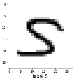
It can be clearly seen that although the true value of 1670 items is 5, it does not look much like 5, a little like 3. Even manual identification has some difficulties.
conclusion
This chapter builds the simplest model of MNIST handwritten data set recognition through multi-layer perceptron. The accuracy of MNIST handwritten data set can reach 0.97 under the test set, which is a good achievement. However, there are over-fitting and a small part of errors in the training model process. The next chapter will describe how to eliminate the over-fitting problem and how to eliminate the over-fitting problem. Further improve the accuracy of the model.