Common probability distribution and hypothesis test

1 general random variable

1.1 two types of random variables

According to the number of possible values of random variables, they are divided into discrete type (finite value) and continuous type (infinite value).

1.2 discrete random variables

For discrete random variables, the probability mass function (PMF) is used to describe their distribution law.

It is assumed that the discrete random variable X has n values, X 1 X_1 X1, X 2 X_2 X2, ..., X n X_n Xn, so
P ( X = X i ) ≥ 0 P(X=X_i) \geq 0 P(X=Xi)≥0

Σ 1 n P ( X = X n ) = 1 \Sigma_{1}^{n} P(X=X_n) =1 Σ1nP(X=Xn)=1

Examples of using PMF: binomial distribution, Poisson distribution

1.3 continuous random variable

For continuous random variables, probability density function (PDF) is used to describe their distribution.

The characteristic of continuous random variable is that the probability of taking any fixed value is 0, so it is meaningless to discuss its probability on a specific value. We should discuss its probability in a certain interval, which uses the concept of probability density function.

It is assumed that the continuous random variable X, f(x) is a probability density function. For any real number range, such as [a,b], there is
P { a ≤ X ≤ b } = ∫ a b f ( x ) d x P \lbrace a\leq X \leq b\rbrace = \int ^b_a f(x) {\rm d}x P{a≤X≤b}=∫abf(x)dx
Examples of using PDF: uniform distribution, normal distribution, exponential distribution

For continuous random variables, the cumulative distribution function (CDF) is usually used to describe its properties. Mathematically, CDF is the integral form of PDF.

The function value of the distribution function F(x) at point X represents the probability that x falls within the interval (− ∞, x]. Therefore, the distribution function is an ordinary function with the definition domain of R. therefore, we can transform the probability problem into a function problem, so we can use the ordinary function knowledge to study the probability problem and increase the research scope of probability.

2 common distribution

This section uses some practical examples to understand various distributions and their application scenarios

2.1 discrete distribution

2.1.1 Binomial distribution

Binomial distribution can be considered as a distribution probability of the number of success times after a single test with only two results (success / failure).

The binomial distribution needs to meet the following conditions:

The number of tests is fixed
Each test is independent
The probability of success is the same for each trial

Some examples of binomial distribution:

Number of successful sales calls
Number of defective products in a batch
The number of times a coin is tossed face up
The number of times to eat candy in a bag of candy and get the red package

In n tests, if the success rate of a single test is p and the failure rate is q=1-p, the probability of success times is
P ( X = x ) = C n x p x q n − x P(X=x) = C_n^x p^x q^{n-x} P(X=x)=Cnxpxqn−x

2.1.2 Poisson distribution

Poisson distribution is a distribution used to describe Poisson test. Tests meeting the following two characteristics can be considered as Poisson test:

The events investigated have equal opportunities to occur once in any two intervals of equal length
Whether the investigated events occur in any interval and whether they occur in other intervals do not affect each other, that is, they are independent

Poisson distribution needs to meet some conditions:

The number of tests n tends to infinity
The probability p of a single event tends to 0
np is a finite number

Some examples of Poisson distribution:

Number of booking calls received by an airline in a certain period of time
The number of people waiting for the bus at the station within a certain period of time
Number of defects found on a piece of cloth
The number of typos in a certain number of pages

A random variable X that obeys Poisson distribution has a rate parameter λ ( λ= In a fixed time interval of np), the probability that the number of events is i is
P { X = i } = e − λ λ i i ! P\lbrace X= i \rbrace = e^{-λ} \frac{λ^i}{i!} P{X=i}=e−λi!λi

2.1.3 relationship between binomial distribution, Poisson distribution and normal distribution

There is a very subtle correlation between these three distributions.

When n is large and p is small, such as n ≥ 100 and np ≤ 10, the binomial distribution can be approximately Poisson distribution.

When λ When very large, such as λ When ≥ 1000, Poisson distribution can be approximately normal distribution.

When n is large, np and n(1-p) are large enough, such as n ≥ 100, np ≥ 10, n(1-p) ≥ 10, the binomial distribution can be approximately normal.

2.1.4 other discrete random distributions

In addition to binomial distribution and Poisson distribution, there are some other less commonly used discrete distributions.

Geometric distribution

Considering the independent repeated test, the geometric distribution describes the probability of first success after k tests, assuming that the success rate of each test is p,
P { X = n } = ( 1 − p ) n − 1 p P\lbrace X= n \rbrace = {(1-p)}^{n-1} p P{X=n}=(1−p)n−1p

Negative binomial distribution

Considering the independent repeated test, the negative binomial distribution describes the probability of the test until r times of success, assuming that the success rate of each time is p,
P { X = n } = C n − 1 r − 1 p r ( 1 − p ) n − r P\lbrace X= n \rbrace = C_{n-1}^{r-1} p^r {(1-p)}^{n-r} P{X=n}=Cn−1r−1pr(1−p)n−r

Hypergeometric Distribution

Hypergeometric distribution describes the sampling with return in a population with a total number of N, in which k elements belong to one group and the remaining N-k elements belong to another group. It is assumed that N times are extracted from the population, including x, and the probability of the first group is
P { X = n } = C k x C N − k n − x C N n P\lbrace X= n \rbrace = \frac {C_{k}^{x} C_{N-k}^{n-x}} {C_{N}^{n}} P{X=n}=CNnCkxCN−kn−x

2.2 continuous distribution

2.2.1 Uniform distribution

Uniform distribution refers to a kind of statistical distribution in which the probability density function is equal everywhere in the definition domain.

If X obeys the uniform distribution on the interval [a,b], it is recorded as X~U[a,b].

The probability density function of uniform distribution X is
f ( x ) = { 1 b − a , a ≤ x ≤ b 0 , o t h e r s f(x)= \begin{cases} \frac {1} {b-a} , & a \leq x \leq b \\ 0, & others \end{cases} f(x)={b−a1,0,a≤x≤bothers
The distribution function is
F ( x ) = { 0 , x < a ( x − a ) ( b − a ) , a ≤ x ≤ b 1 , x > b F(x)=\begin{cases} 0 , & x< a \\ (x-a)(b-a), & a \leq x \leq b \\ 1, & x>b \end{cases} F(x)=⎩⎪⎨⎪⎧0,(x−a)(b−a),1,x<aa≤x≤bx>b
Some examples of uniform distribution:

An ideal random number generator
The angle at which an ideal disk is stationary after rotating with a certain force

2.2.2 Normal distribution

Normal distribution, also known as Gaussian distribution, is one of the most common statistical distributions. It is a symmetrical distribution. The probability density presents the shape of a pendulum, and its probability density function is
f ( x ) = 1 2 π σ e − ( x − u ) 2 2 σ 2 f(x)=\frac{1}{\sqrt{2π}\sigma}e^{\frac{-(x-u)^2}{2\sigma^2}} f(x)=2π σ1e2σ2−(x−u)2
Marked as x ~ n( μ, σ 2 σ^2 σ 2) , where μ Is the mean of normal distribution, σ Is the standard deviation of normal distribution

With the general normal distribution, it can be transformed into the standard normal distribution Z ~ N(0,1) by formula transformation,
Z = X − μ σ Z=\frac {X-μ} {σ} Z=σX−μ
Some examples of normal distribution:

Adult height
Velocity of gas molecules in different directions
Error in measuring object mass

There are many examples of normal distribution in real life, which can be explained by the central limit theorem. The central limit theorem says that the average value of a group of independent and identically distributed random samples is approximately normal distribution, no matter what distribution the population of random variables conforms to.

2.2.3 Exponential distribution

Exponential distribution is usually widely used to describe the time required for a specific event. In the distribution of exponential random variables, there are few large values and many small values.

The probability density function of exponential distribution is
f ( x ) = { λ e − λ x , x ≥ 0 0 , x < 0 f(x)= \begin{cases} λe^{-λx} , & x \geq 0 \\ 0, & x < 0 \end{cases} f(x)={λe−λx,0,x≥0x<0
Record as X~E( λ), among λ It is called rate parameter, which indicates the number of times the event occurs per unit time.

The distribution function is
F ( a ) = P { X ≤ a } = 1 − e − λ a , a ≥ 0 F(a) = P\{X \leq a\} = 1-e^{-λa}, a\geq 0 F(a)=P{X≤a}=1−e−λa,a≥0
Some examples of exponential distribution:

The time interval between customers arriving at a store
The time interval between now and the earthquake
Time interval between receiving a problem product on the production line

Another interesting property about the exponential distribution is that the exponential distribution is memoryless. It is assumed that some time has passed in the process of waiting for the occurrence of the event. At this time, the distribution of the time interval from the occurrence of the next event is exactly the same as at the beginning, just as the waiting period did not occur at all, and it will not have any impact on the results, To express it in mathematical language is
P { X > s + t ∣ X > t } = P { X > s } P\{X>s+t | X> t\} =P\{X>s\} P{X>s+t∣X>t}=P{X>s}

2.2.4 other continuous distributions

Γ \Gamma Γ distribution

It is often used to describe the distribution of waiting time for an event to occur n times in total

Weibull distribution

It is often used to describe the life of a class of objects with "weakest chain" in the engineering field

2.3 summary of mean and variance of common distributions

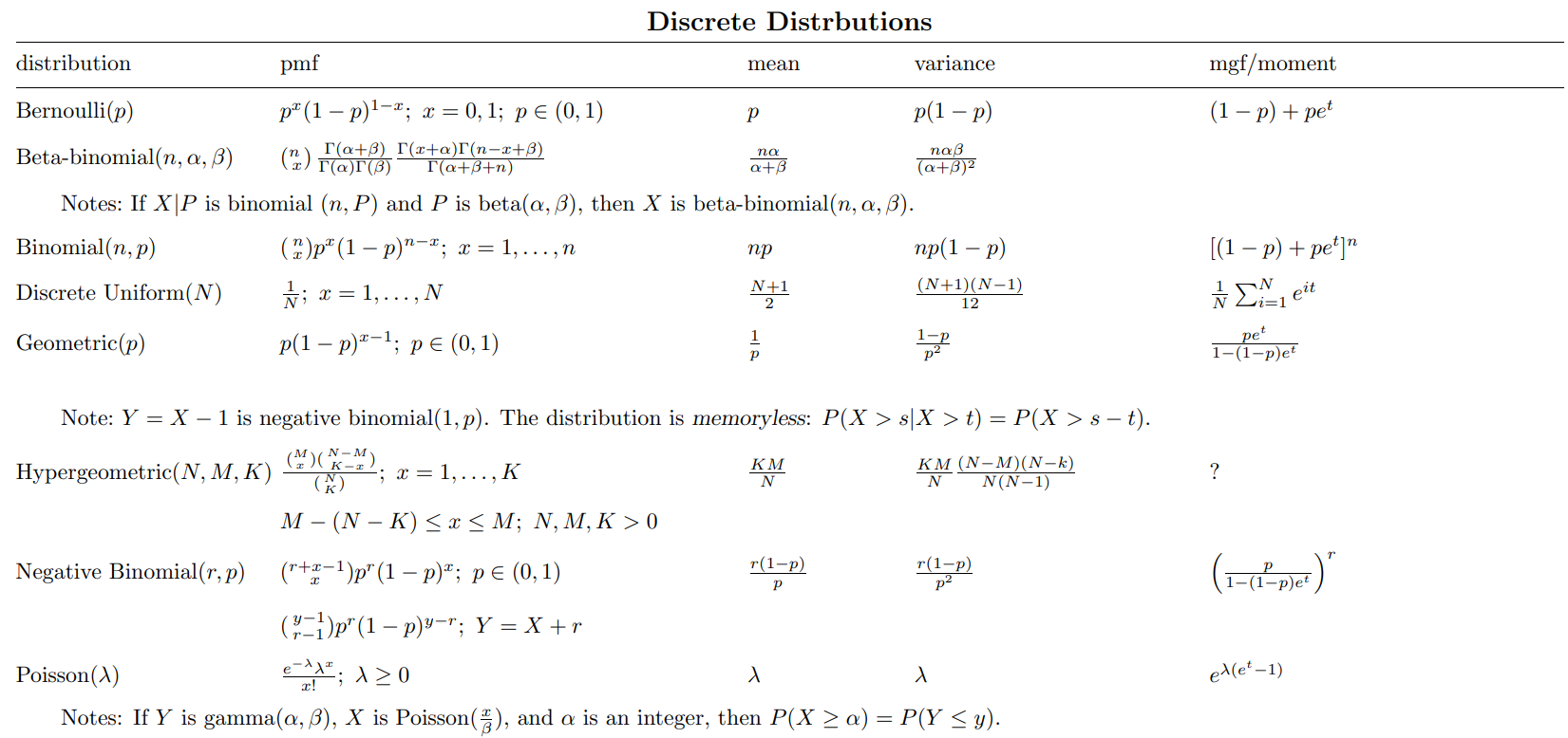
Discrete distribution

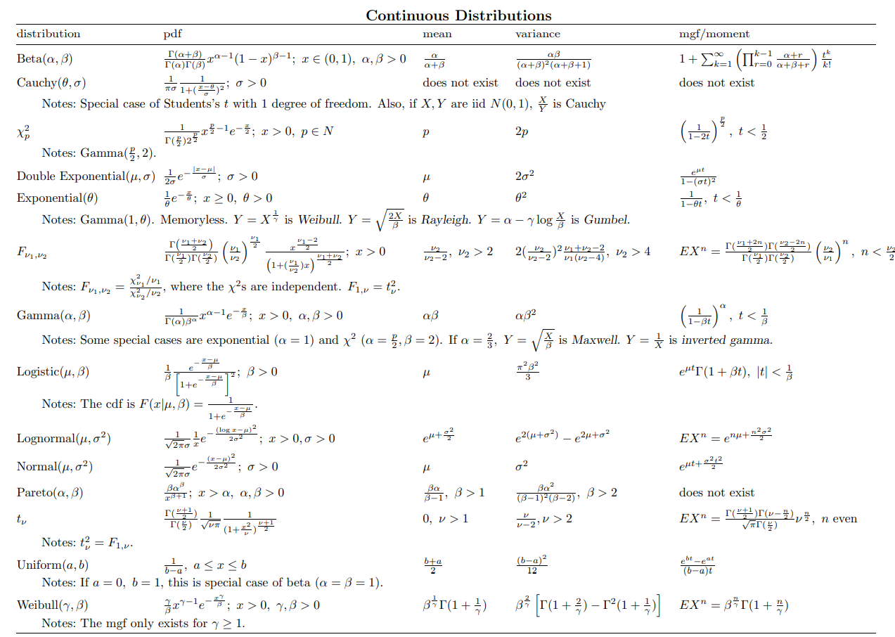
Continuous distribution

2.4 Python code practice

2.4.1 generate a set of random numbers conforming to a specific distribution

In the Numpy library, a set of random classes is provided to generate random numbers with specific distribution

import numpy

# Generate a sample set with a size of 1000 conforming to the b(10,0.5) binomial distribution
s = numpy.random.binomial(n=10,p=0.5,size=1000)

# Generate a sample set conforming to the Poisson distribution of P(1) with a size of 1000
s = numpy.random.poisson(lam=1,size=1000)

# Generate a sample set with a size of 1000 that conforms to the uniform distribution of U(0,1). Note that the boundary value in this method is the left closed right open interval
s = numpy.random.uniform(low=0,high=1,size=1000)

# Generate a sample set conforming to N(0,1) normal distribution with a size of 1000. You can use normal function to customize the mean and standard deviation, or directly use standard_normal function
s = numpy.random.normal(loc=0,scale=1,size=1000)
s = numpy.random.standard_normal(size=1000)

# Generate a sample set with a size of 1000 conforming to E(1/2) exponential distribution. Note that the parameters in this method are exponential distribution parameters λ Reciprocal of
s = numpy.random.exponential(scale=2,size=1000)

In addition to Numpy, Scipy also provides a set of methods for generating specific distributed random numbers

# Taking uniform distribution as an example, rvs can be used to generate the values of a set of random variables
from scipy import stats
stats.uniform.rvs(size=10)

2.4.2 PMF and PDF for calculating statistical distribution

The Scipy library provides a set of methods for calculating discrete random variable PMF and continuous random variable PDF.

from scipy import stats

# Calculate the PMF of binomial distribution B(10,0.5)
x=range(11)
p=stats.binom.pmf(x, n=10, p=0.5)

# Calculate the PMF of Poisson distribution P(1)
x=range(11)
p=stats.poisson.pmf(x, mu=1)

# Calculate PDF of uniformly distributed U(0,1)
x = numpy.linspace(0,1,100)
p= stats.uniform.pdf(x,loc=0, scale=1)

# Calculate PDF of normal distribution N(0,1)
x = numpy.linspace(-3,3,1000)
p= stats.norm.pdf(x,loc=0, scale=1)

# PDF for calculating exponential distribution E(1)
x = numpy.linspace(0,10,1000)
p= stats.expon.pdf(x,loc=0,scale=1)

2.4.3 calculate the CDF of statistical distribution

Similar to the method of calculating probability mass / density function, the value of distribution function can be obtained by replacing pmf or pdf in the previous section with cdf

# Taking the normal distribution as an example, the CDF of normal distribution N(0,1) is calculated
x = numpy.linspace(-3,3,1000)
p = stats.norm.cdf(x,loc=0, scale=1)

2.4.4 visualization of statistical distribution

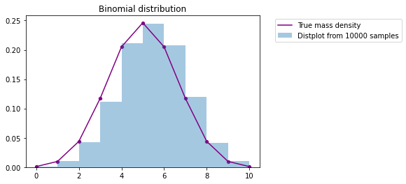
Binomial distribution

The real probability quality of binomial distribution with n=10 and p=0.5 and the results of 10000 random samples are compared

from scipy import stats
import matplotlib.pyplot as plt
import seaborn as sns

x = range(11)  # Number of successful binomial distribution (X-axis)
t = stats.binom.rvs(10,0.5,size=10000) # B(10,0.5) 10000 random samples
p = stats.binom.pmf(x, 10, 0.5) # B(10,0.5) real probability quality

fig, ax = plt.subplots(1, 1)
sns.distplot(t,bins=10,hist_kws={'density':True}, kde=False,label = 'Distplot from 10000 samples')
sns.scatterplot(x,p,color='purple')
sns.lineplot(x,p,color='purple',label='True mass density')
plt.title('Binomial distribution')
plt.legend(bbox_to_anchor=(1.05, 1))

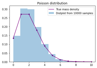
Poisson distribution

compare λ= The real probability quality of Poisson distribution and the results of 10000 random samples

from scipy import stats
import matplotlib.pyplot as plt
import seaborn as sns
x=range(11)
t= stats.poisson.rvs(2,size=10000)
p=stats.poisson.pmf(x, 2)

fig, ax = plt.subplots(1, 1)
sns.distplot(t,bins=10,hist_kws={'density':True}, kde=False,label = 'Distplot from 10000 samples')
sns.scatterplot(x,p,color='purple')
sns.lineplot(x,p,color='purple',label='True mass density')
plt.title('Poisson distribution')
plt.legend()

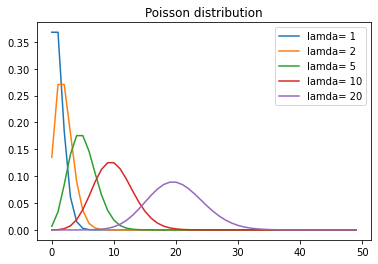
x=range(50)
fig, ax = plt.subplots()
for  lam in [1,2,5,10,20] :
        p=stats.poisson.pmf(x, lam)
        sns.lineplot(x,p,label='lamda= '+ str(lam))
plt.title('Poisson distribution')
plt.legend()

uniform distribution

Compare the real probability density of uniform distribution of U(0,1) with the results of 10000 random samples

from scipy import stats
import matplotlib.pyplot as plt
import seaborn as sns
x=numpy.linspace(0,1,100)
t= stats.uniform.rvs(0,1,size=10000)
p=stats.uniform.pdf(x, 0, 1)

fig, ax = plt.subplots(1, 1)
sns.distplot(t,bins=10,hist_kws={'density':True}, kde=False,label = 'Distplot from 10000 samples')

sns.lineplot(x,p,color='purple',label='True mass density')
plt.title('Uniforml distribution')
plt.legend(bbox_to_anchor=(1.05, 1))

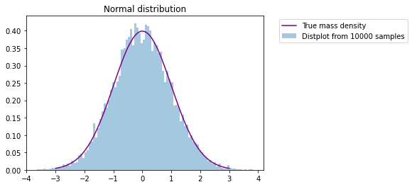
Normal distribution

Compare the true probability density of the normal distribution of N(0,1) with the results of 10000 random samples

from scipy import stats
import matplotlib.pyplot as plt
import seaborn as sns
x=numpy.linspace(-3,3,100)
t= stats.norm.rvs(0,1,size=10000)
p=stats.norm.pdf(x, 0, 1)

fig, ax = plt.subplots(1, 1)
sns.distplot(t,bins=100,hist_kws={'density':True}, kde=False,label = 'Distplot from 10000 samples')


sns.lineplot(x,p,color='purple',label='True mass density')
plt.title('Normal distribution')
plt.legend(bbox_to_anchor=(1.05, 1))

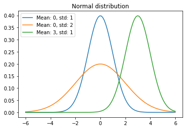
Compare the probability density function of normal distribution with different combinations of mean and standard deviation

x=numpy.linspace(-6,6,100)
p=stats.norm.pdf(x, 0, 1)
fig, ax = plt.subplots()
for  mean, std in [(0,1),(0,2),(3,1)]: 
        p=stats.norm.pdf(x, mean, std)
        sns.lineplot(x,p,label='Mean: '+ str(mean) + ', std: '+ str(std))
plt.title('Normal distribution')
plt.legend()

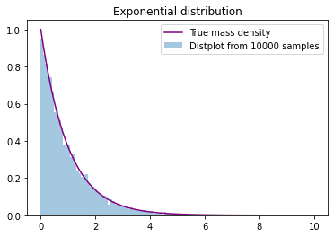
exponential distribution

Compare the real probability density of the exponential distribution of E(1) with the results of 10000 random samples

from scipy import stats
import matplotlib.pyplot as plt
import seaborn as sns
x=numpy.linspace(0,10,100)
t= stats.expon.rvs(0,1,size=10000)
p=stats.expon.pdf(x, 0, 1)

fig, ax = plt.subplots(1, 1)
sns.distplot(t,bins=100,hist_kws={'density':True}, kde=False,label = 'Distplot from 10000 samples')


sns.lineplot(x,p,color='purple',label='True mass density')
plt.title('Exponential distribution')
plt.legend(bbox_to_anchor=(1, 1))

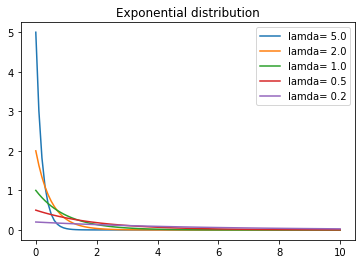
Compare the probability density function of exponential distribution with different parameters

x=numpy.linspace(0,10,100)
fig, ax = plt.subplots()
for  scale in [0.2,0.5,1,2,5] :
        p=stats.expon.pdf(x, scale=scale)
        sns.lineplot(x,p,label='lamda= '+ str(1/scale))
plt.title('Exponential distribution')
plt.legend()

3 hypothesis test

3.1 basic concepts

Hypothesis testing is an important problem in statistical inference. When the distribution function of the population is completely unknown or only its form and parameters are known, some assumptions about the population are put forward in order to infer some unknown characteristics of the population. This kind of problem is called hypothesis testing.

3.2 basic steps

A hypothesis testing problem can be divided into five steps, which will be followed no matter how the details change.

State the research hypothesis, including null hypothesis and alternative hypothesis
Collect (sample) data for hypothesis validation
Construct appropriate statistical test quantity and test
Decide whether to reject the original hypothesis
Show conclusion

Step 1:

Generally speaking, we will describe the original hypothesis as that there is no difference or correlation between variables, and the alternative hypothesis is that there is a difference or correlation.

For example, the original hypothesis is that there is no difference in the average height between men and women, and the alternative hypothesis is that there is a significant difference in the average height between men and women.

Step 2:

In order to make the statistical test results true and reliable, samples should be taken from the population according to the actual hypothetical proposition, and the sampling data should be representative. For example, in the above proposition of average height of men and women, the samples should cover all social classes, countries and other factors that may affect height.

Step 3:

There are many kinds of statistical tests, but all statistical tests are based on the comparison of intra group variance and inter group variance. If the inter group variance is large enough so that there is little overlap between different groups, the statistics will reflect a very small P value, which means that the differences between different groups cannot be caused by chance.

Step 4:

Based on the results of statistics, we make a judgment that we cannot reject the original hypothesis or reject the original hypothesis. Usually, we will take P=0.05 as the critical value (one-sided test).

Step 5:

Show the conclusion.

3.3 selection of Statistics

Selecting appropriate statistics is the key step of hypothesis testing. The most commonly used statistical tests include regression test, comparison test and correlation test.

Regression test

Regression test is applicable to the case where the prediction variables are numerical. According to the number of prediction variables and the type of result variables, it can be divided into the following categories.

	Predictive variable	Result variable
Simple linear regression	Single, continuous value	Continuous value
Multiple linear regression	Multiple, continuous values	Continuous value
Logistic regression	Continuous value	Binary category

Comparative test

The comparison test is applicable to the case where the prediction variable is of category type and the result variable is of numerical type. It can be divided into the following types according to the number of groups of prediction variables and the number of result variables.

	Predictive variable	Result variable
Paired t-test	Two groups, category	Group from the same population, numerical
Independent t-test	Two groups, category	Groups from different populations, values
ANOVA	Two or more groups, category	Single, numeric
MANOVA	Two or more groups, category	Two or more values

Correlation test

Only chi square test is commonly used in correlation test, which is applicable to the case where both predictive variables and outcome variables are category type.

Nonparametric test

In addition, generally speaking, the above parameter tests need to meet some preconditions, the samples are independent, and the intra group variance approximation and data of different groups meet normality. Therefore, when these conditions are not met, we can try to replace the parameter test with nonparametric test.

Nonparametric test	Parameter verification for substitution
Spearman	Regression and correlation test
Sign test	T-test
Kruskal–Wallis	ANOVA
ANOSIM	MANOVA
Wilcoxon Rank-Sum test	Independent t-test
Wilcoxon Signed-rank test	Paired t-test

3.4 two types of errors

In fact, it is possible for us to make mistakes in the process of hypothesis testing, and in theory, mistakes can not be completely avoided. By definition, errors are divided into two types: type I error and type II error.

A kind of error: rejecting the true original hypothesis
Type II error: accept the wrong original hypothesis

A type of error can be passed α Value to control the choice in the hypothesis test α (significance level) has a direct impact on a class of errors. α It can be considered that we are the most likely to make a kind of mistake. Taking the 95% confidence level as an example, a=0.05, which means that the probability of rejecting a true original hypothesis is 5%. In the long run, every 20 hypothesis tests, there will be an event of making a kind of mistake.

Class II errors are usually caused by small samples or high sample variance. The probability of class II errors can be used β Different from a class of errors, such errors cannot be directly controlled by setting an error rate. For class II errors, it can be estimated from the perspective of efficacy. Firstly, power analysis is carried out to calculate the efficacy value 1- β， Then the estimation of class II error is obtained β.

Generally speaking, these two types of errors cannot be reduced at the same time. On the premise of reducing the possibility of making class I errors, it will increase the possibility of making class II errors. How to balance these two types of errors in actual cases depends on whether we are more able to accept class I errors or class II errors.

3.5 Python code practice

This section uses some examples to explain how to use python for hypothesis testing.

3.5.1 normal test

Shapiro Wilk test is a classical normal test method.

H0: the sample population obeys normal distribution

H1: the sample population does not obey the normal distribution

import numpy as np
from scipy.stats import shapiro
data_nonnormal = np.random.exponential(size=100)
data_normal = np.random.normal(size=100)

def normal_judge(data):
	stat, p = shapiro(data)
	if p > 0.05:
		return 'stat={:.3f}, p = {:.3f}, probably gaussian'.format(stat,p)
	else:
		return 'stat={:.3f}, p = {:.3f}, probably not gaussian'.format(stat,p)

# output
normal_judge(data_nonnormal)
# 'stat=0.850, p = 0.000, probably not gaussian'
normal_judge(data_normal)
# 'stat=0.987, p = 0.415, probably gaussian'

3.5.2 chi square test

Objective: to test whether the two groups of category variables are related or independent

H0: the two samples are independent

H1: the two groups of samples are not independent

from scipy.stats import chi2_contingency
table = [[10, 20, 30],[6,  9,  17]]
stat, p, dof, expected = chi2_contingency(table)
print('stat=%.3f, p=%.3f' % (stat, p))
if p > 0.05:
	print('Probably independent')
else:
	print('Probably dependent')

 # output
#stat=0.272, p=0.873
#Probably independent

3.5.3 T-test

Objective: to test whether the mean values of two independent sample sets have significant differences

H0: the mean is equal

H1: the mean value is unequal

from scipy.stats import ttest_ind
import numpy as np
data1 = np.random.normal(size=10)
data2 = np.random.normal(size=10)
stat, p = ttest_ind(data1, data2)
print('stat=%.3f, p=%.3f' % (stat, p))
if p > 0.05:
	print('Probably the same distribution')
else:
	print('Probably different distributions')
    
# output
# stat=-1.382, p=0.184
# Probably the same distribution

3.5.4 ANOVA

Objective: similar to t-test, ANOVA can test whether there are significant differences in the mean values of two or more independent sample sets