The use of residual network in CNN
- K. He, X. Zhang, S. Ren and J. Sun, "Deep Residual Learning for Image Recognition," in 2016 IEEE Conference on Computer Vision and Pattern Recognition (CVPR), Las Vegas, NV, USA, 2016 pp. 770-778.doi: 10.1109/CVPR.2016.90
-
Innovation:
- The residual network still makes the non-linear layer satisfy H(x,wh)H(x,w_h)H(x,wh) (mapping relationship of ordinary network), and then directly introduce a short connection from the input to the output of non-linear layer, so that the whole mapping becomes:
y=H(x,wh)+x y=H(x,w_h)+x y=H(x,wh)+x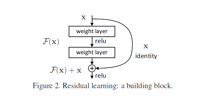
F (x) = H (x, wh) f (x) = H (x, w)_ h)F(x)=H(x,wh).
- The residual network still makes the non-linear layer satisfy H(x,wh)H(x,w_h)H(x,wh) (mapping relationship of ordinary network), and then directly introduce a short connection from the input to the output of non-linear layer, so that the whole mapping becomes:
-
advantage
- On the one hand, the residual network can better fit the classification function to obtain higher classification accuracy. This theory gives a very reasonable inspiration, that is, in principle, the ability of fitting the high-dimensional function of the network with short connection is stronger than that of the network with ordinary connection. ResNet not only increases the depth of the network, but also does not increase the complexity of the network, and the effect is much better than other networks such as VGG and Google net. With the increase of the number of layers, this advantage is more and more obvious.
- The residual network solves the problem of optimizing training when the number of layers of the network is deepened (short link).
- Identity mapping does not bring extra parameters and computation to the model.
-
inferiority:
Two kinds of Shortcut connections are introduced. The first is used in the case of equal dimension when adding features, that is, identity mapping. Obviously, the second is used in the case of unequal.
- Identity mapping does not bring extra parameters and computation to the model. However, using shortcut connections without parameters requires that the dimensions of X and F(x) are equal, otherwise they cannot be added.
- When dimensions are not equal, a match is required.
-
reason:
-
Network characteristics: in some application areas, deep network is very important. However, deep-level networks are difficult to train and are prone to gradient disappearance or gradient explosions. However, these problems have been basically solved through normalized initialization and intermediate normalization layers (BN layer), so that the network can reach dozens of layers of depth, and can be effectively trained using back propagation algorithm. However, when the deeper network begins to converge, a problem called "degradation problem of training accuracy" is exposed: with the increase of network depth, the accuracy on the training set reaches saturation, and then drops rapidly.
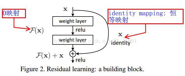
As shown in the figure, X is the input, F(x) is the output of general neural network, X is a quick connection of identity mapping, and ReLu is the activation function. So why do degradation problems arise, that is, deeper networks cannot guarantee performance at least equivalent to that of shallower networks? If we remove the fast connection x, we want to ensure that x forms identity map through the weight layer, then F(x) = H(x) =x, where H(x) is the potential map that the network wants to fit. Facts show that the optimization of this process is very difficult. For example, when x = 10, F(x) = 10.1, the rate of change is (10.1-10) / 10 = 1%; when we add quick link, H(x)=F(x)+x, H(x)=10.1, F(x) =10.1-10= 0.1, the rate of change is (0.1-10) / 10 ≈ 100%. This is very good for the adjustment of weight, forcing the weight to approach 0, so F(x) is optimized to 0, at this time H(x) =x, identity mapping is completed. In real training, the weight can not be close to 0 completely, and F(x) can only approach 0. To sum up, when a network is trained to a certain extent and the accuracy is not improved, we can link the residual network, because the latter is almost the identity map, and the error of this method will not be greater than that of the shallow network, and the network can continue to be optimized to improve the network performance.In other words, after we join the fast connection, the original identity map becomes zero map, and the network is easier to optimize. Reference article 1
-
**Scene features: * * target detection, image segmentation.
-
code:
import torch
import torch.nn as nn
from torch.utils.data import DataLoader
from torchvision import transforms
from torchvision import datasets  # Many common data sets are placed, including handwritten digit recognition
import torch.nn.functional as F
Data preprocessing
transform = transforms.Compose([
    transforms.ToTensor(),  # Rotation tensor, reduce the value to [0,1]
    transforms.Normalize((0.1307,),(0.3081,))  # Normalization, the first is the mean, the second is the variance
])
# Load data
train_dataset = datasets.MNIST(root= "E:/MNIST/mnist",
                              train=True,  # Download training set
                              transform=transform,  # Transtensor, reduce the value to [0,1]. It can also be written as transform= transforms.ToTensor ()
                              download=True
                              )

test_dataset = datasets.MNIST(root= "E:/MNIST/mnist",
                              train=False,  # Download training set
                              transform=transform,  # Rotation tensor, reduce the value to [0,1]
                              download=True
                              )

train_loader = DataLoader(dataset=train_dataset,
                         batch_size=64,
                         shuffle=True)
test_loader = DataLoader(dataset=test_dataset,
                         batch_size=64,
                         shuffle=False)
Residual Block
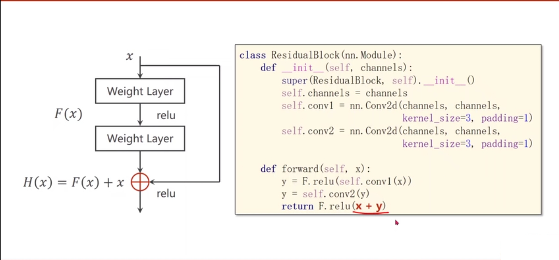
class ResidualBlock(nn.Module):
    def __init__(self, channels):
        super(ResidualBlock, self).__init__()
        self.channels = channels
        self.conv1 = nn.Conv2d(channels, channels, kernel_size=3, padding = 1)
        self.conv2 = nn.Conv2d(channels, channels, kernel_size=3, padding = 1)
    # The residual network is used once for two convolutional layers.
    def forward(self, x):
        y = F.relu(self.conv1(x))
        y = self.conv2(y)
        return F.relu(x+y)  # First sum and then activate.
Building CNN model
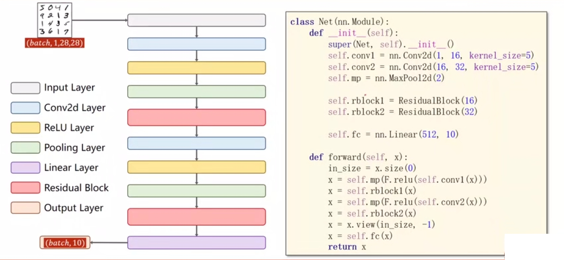
class Net(nn.Module):
    def __init__(self):
        super(Net,self).__init__()
        self.conv1 = nn.Conv2d(1, 16, kernel_size=5)
        self.conv2 = nn.Conv2d(16, 32, kernel_size=5)
        self.mp = nn.MaxPool2d(2)

        self.rblock1 = ResidualBlock(16)
        self.rblock2 = ResidualBlock(32)

        self.fc = nn.Linear(512, 10)

    def forward(self, x):  # (batch_size, channel, W, H)
        in_size = x.size(0)  # batch_size
        x = self.mp(F.relu(self.conv1(x)))
        x = self.rblock1(x)
        x = self.mp(F.relu(self.conv2(x)))
        x = self.rblock2(x)
        x = x.view(in_size, -1)
        x = self.fc(x)
        return x
model = Net()
loss_fn = torch.nn.CrossEntropyLoss()
optimizer = torch.optim.SGD(model.parameters(), lr= 0.01, momentum= 0.5)
Training function
def train(epoch):
    runing_loss = 0.0
    for batch_idx, data in enumerate(train_loader, 0):
        inputs, target =data
        inputs, target = inputs.to(device), target.to(device)
        optimizer.zero_grad()

        outputs = model(inputs)
        loss = loss_fn(outputs, target)
        loss.backward()
        optimizer.step()

        runing_loss += loss.item()
        if batch_idx % 300  == 299:
            print("[%d, %5d] loss: %.3f" % (epoch +1, batch_idx+1, runing_loss/300))
            runing_loss = 0.0
Test function
def test():
    correct = 0
    total =0
    with torch.no_grad():
        for data in test_loader:
            images, labels =data
            outputs = model(images)
            _, predicted = torch.max(outputs.data, dim =1 )  # Returns two values, the first is the maximum value and the second is the index of the maximum value. dim=1 indicates the above results in column dimension, and dim = 0 indicates the above results in row dimension.
            total += labels.size(0)  # Every batch_ In size, labels is a tuple of (N, 1), size(0)=N
            correct +=(predicted == labels).sum().item()  # Total number of yes
    print("Accuracy on the test set %d %%" % (100*correct/total))
Network start
if __name__=="__main__":
    for epoch in range(10):
        train(epoch)
        if epoch % 2 ==0:
            test()
[1,   300] loss: 0.535
[1,   600] loss: 0.165
[1,   900] loss: 0.121
Accuracy on the test set 96 %
[2,   300] loss: 0.085
[2,   600] loss: 0.088
[2,   900] loss: 0.077
[3,   300] loss: 0.060
[3,   600] loss: 0.060
[3,   900] loss: 0.060
Accuracy on the test set 98 %
[4,   300] loss: 0.046
[4,   600] loss: 0.052
[4,   900] loss: 0.047
[5,   300] loss: 0.039