preface
Although the code is often very long, it is annotation for understanding
1, KMeans
KMeans can be said to be one of the simplest clustering algorithms
1.1 how does kmeans work
Key concepts: cluster and centroid
- KMeans algorithm divides the characteristic matrix X of a group of N samples into K clusters without intersection. Intuitively, the cluster is a group of data gathered together, and the data in a cluster is considered to be the same class. Cluster is the result of clustering.
- Mean of all data in the cluster μ i \mu_i μ i) is often referred to as the "centroids" of this cluster. In a two-dimensional plane, the abscissa of the centroid of a cluster of data points is the mean of the abscissa of the cluster of data points, and the ordinate of the centroid is the mean of the ordinate of the cluster of data points. The same principle can be extended to high-dimensional space.
In KMeans algorithm, the number of clusters K is a super parameter, which needs to be determined by human input. The core task of KMeans is to find K optimal centroids according to the K we set, and assign the data closest to these centroids to the clusters represented by these centroids. The specific process can be summarized as follows:
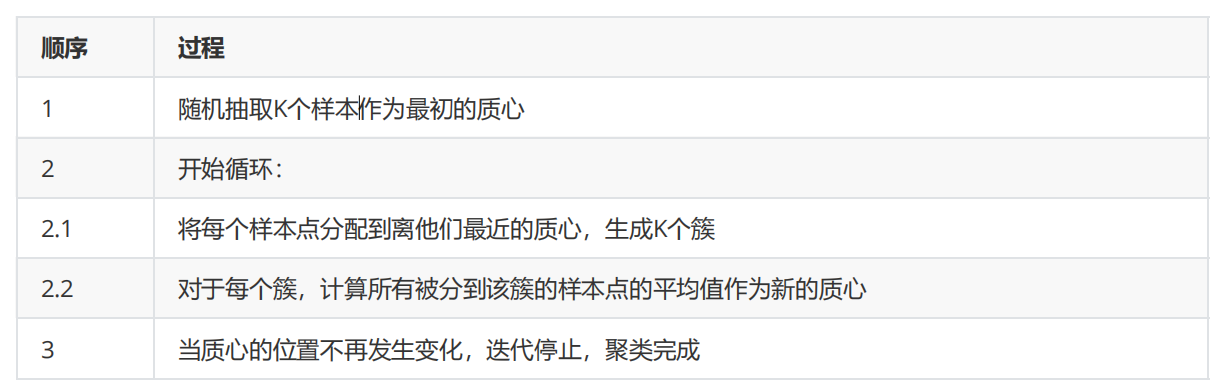
When we find a centroid, the samples assigned to this centroid in each iteration are consistent, that is, the newly generated clusters are consistent every time. All sample points will not be transferred from one cluster to another, and the centroid will not change.
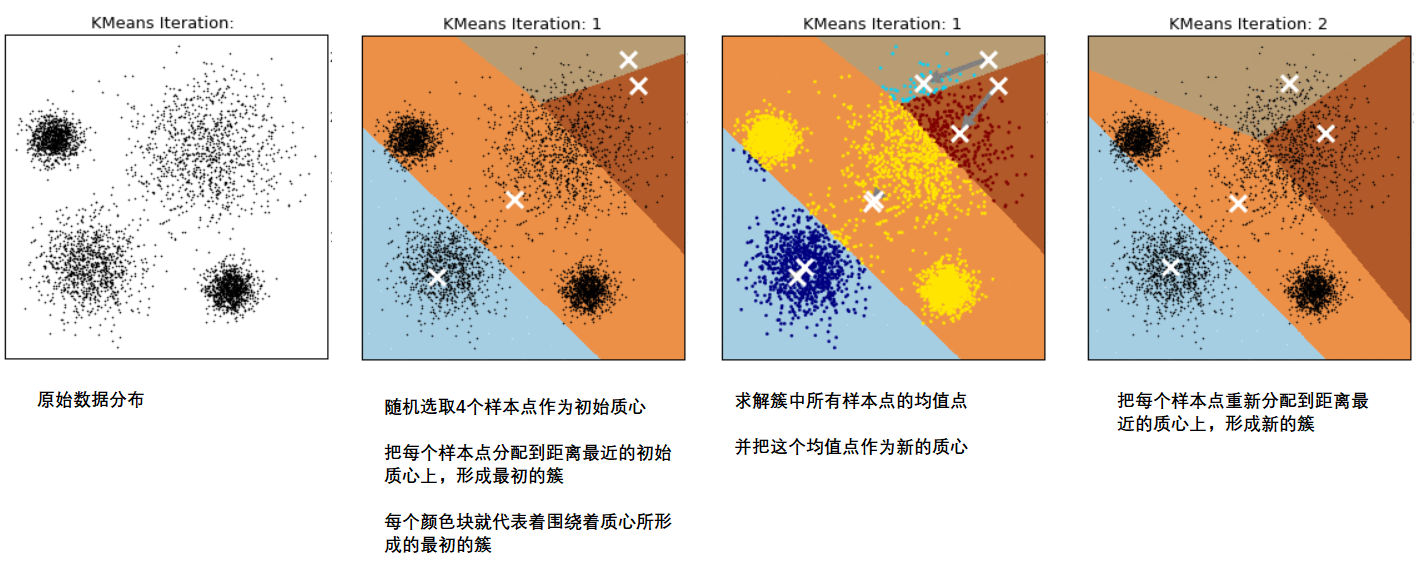
This process can be shown in the following figure. We specify that the data are divided into 4 clusters (K=4), where white X represents the position of the centroid:
1.2 sum of squares of intra cluster errors
The data in the same cluster are similar, while the data in different clusters are different
After clustering, we have to study the properties of the samples in each cluster, so as to formulate different business or technology strategies according to business needs. This sounds like Scorecard case The concept of "box division" explained is somewhat similar, that is, our purpose of box division is to hope that people in one box have similar credit risks, while people in different boxes have huge differences in credit risks, so as to distinguish people with different credit degrees. Therefore, we pursue "small differences within groups and large differences between groups". Clustering algorithm is also the same purpose. We pursue "small difference within the cluster and large difference outside the cluster". This "difference" is measured by the distance from the sample point to the centroid of its cluster.
For a cluster, the smaller the sum of the distances from all sample points to the centroid, we think that the more similar the samples in the cluster, the smaller the difference within the cluster. There are many methods to measure the distance:
Oh
A few
in
have to
distance
leave
:
d
(
x
,
μ
)
=
∑
i
=
1
n
(
x
i
−
μ
i
)
2
Euclidean distance: D (x, \ mu) = \ sqrt {\ sum {I = 1} ^ {n} (x _i - \ mu _i) ^ 2}
Euclidean distance: d(x, μ)= i=1∑n(xi− μ i)2
Man
Ha
Dun
distance
leave
:
d
(
x
,
μ
)
=
∑
i
=
1
n
(
∣
x
i
−
μ
∣
)
Manhattan distance: d(x,\mu)=\sum_{i=1}^{n}(|x_i-\mu|)
Manhattan distance: d(x, μ)= i=1∑n(∣xi− μ ∣)
more than
string
distance
leave
:
cos
θ
=
∑
i
=
1
n
(
x
i
∗
μ
)
∑
i
=
1
n
(
x
i
)
2
∗
∑
i
=
1
n
(
μ
)
2
Cosine distance: \ cos \ theta = \ frac {\ sum {I = 1} ^ {n} (x _i * \ mu)} {\ sqrt {\ sum {I = 1} ^ {n} (x _i) ^ 2} * \ sqrt {\ sum {I = 1} ^ {n} (\ mu) ^ 2}}
Cosine distance: cos θ= ∑i=1n(xi)2
∗∑i=1n(μ)2
∑i=1n(xi∗μ)
- x : x: x: A sample point in a cluster
- μ : \mu: μ: Centroid in the cluster
- n : n: n: Shows the number of features in each sample point
- i : i: i: Composition point x x Each feature of x
If we use Euclidean distance, the sum of squares of the distances from all sample points in a cluster to the centroid is:
C
l
u
s
t
e
r
S
u
m
o
f
S
q
u
a
r
e
(
C
S
S
)
=
∑
j
=
0
m
∑
i
=
1
n
(
x
i
−
μ
i
)
2
Cluster~Sum~of~Square~(CSS)=\sum_{j=0}^{m}\sum_{i=1}^{n}(x_i-\mu_i)^2
Cluster Sum of Square (CSS)=j=0∑mi=1∑n(xi−μi)2
T
o
t
a
l
C
l
u
s
t
e
r
S
u
m
o
f
S
q
u
a
r
e
=
∑
l
=
1
k
C
S
S
l
Total~Cluster~Sum~of~Square=\sum_{l=1}^{k}CSS_l
Total Cluster Sum of Square=l=1∑kCSSl
- m : m: m: Is the number of samples in a cluster
- j : j: j: Number of each sample
This formula is called cluster Sum of Square, also known as Inertia. Adding the sum of squares of all clusters in a data set gives the total cluster Sum of Square, also known as total Inertia. The smaller the total Inertia, the more similar the samples in each cluster, the better the clustering effect.
KMeans seeks to solve the centroid that can minimize Inertia.
In the process of constant change and iteration of the center of mass, the total sum of squares is getting smaller and smaller. We can use mathematics to prove that when the total sum of squares is the smallest, the center of mass will no longer change. In this way, the solution process of K-Means becomes an optimization problem.
In KMeans, under a fixed number of clusters K, we minimize the total square sum to solve the optimal centroid, and cluster based on the existence of the centroid. This is very similar to the process of minimizing the loss function in logistic regression, and the minimum value of the total distance square sum can be solved by gradient descent.
Does KMeans have a loss function
-
There was such a conclusion in logistic regression: the essence of loss function is to measure the fitting effect of the model. Only when there is an algorithm to solve the parameter requirements, there will be loss function.
Kmeans does not solve any parameters, and its model essence is not fitting the data, but exploring the data. Inertia is more like kmeans' model evaluation index than loss function.
-
In contrast, in the decision tree, we have the standard accuracy to measure the classification effect. The loss corresponding to the accuracy is called generalization error, but we can't solve the information required in a model by minimizing the generalization error. We just hope that the generalization error shown in the effect of the model is very small. Therefore, there is absolutely no loss in decision tree, KNN and other algorithms Function.
Inertia is based on the Euclidean distance calculation formula. In fact, we can also use other distances, and each distance has its own inertia. In Kmeans, as long as the correct combination of centroid and distance is used, no matter what distance is used, good clustering effect can be achieved:
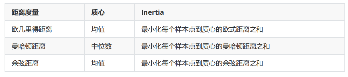
These combinations are derived by strict mathematical proof. In sklearn, we can't choose the distance to use, but can only use the European distance. Therefore, we don't need to worry about how to get the centroid selection of these distances.
1.3 time complexity of kmeans algorithm
In addition to the effect of the model itself, we also use another angle to measure the algorithm: algorithm complexity.
The complexity of the algorithm is divided into time complexity and space complexity. Time complexity refers to the computational workload required to execute the algorithm, which is commonly expressed by large O symbols; and space complexity refers to the memory space required to execute the algorithm.
If the effect of an algorithm is very good, but the time complexity and space complexity are very large, we will weigh the effect of the algorithm and the required computational cost.
Like KNN, KMeans algorithm is a very expensive algorithm.
The average complexity of KMeans algorithm is O(knT), where k is our super parameter, the number of clusters to be input, n is the sample size of the whole data set, and T is the number of iterations required (relatively, the average complexity of KNN is O(n)). In the worst case, the complexity of KMeans can be written O ( n ( k + 2 ) / p ) O(n^{(k+2)/p}) O(n(k+2)/p), where n is the sample size of the whole data set and p is the total number of features.
Compared with other clustering algorithms, k-means algorithm is faster, but it generally finds the local minimum of Inertia. That's why many times
It would be useful to restart it.
2, sklearn.cluster.KMeans
class sklearn.cluster.KMeans (n_clusters=8, init='k-means++', n_init=10, max_iter=300, tol=0.0001,
precompute_distances='auto', verbose=0, random_state=None, copy_x=True, n_jobs=None, algorithm='auto')
2.1 important parameters n_clusters
n_clusters is k in KMeans, which means that we tell the model how many categories we want to divide. This is the only required parameter in KMeans. The default is 8 categories, but usually our clustering result will be a result less than 8. Usually, we don't know n before we start clustering_ How many clusters are, so we should explore it.
2.1.1 design primary clustering
When we get a data set, if possible, we hope to observe the data distribution of the data set through drawing, so as to provide the N input during clustering_ Clusters as a reference.
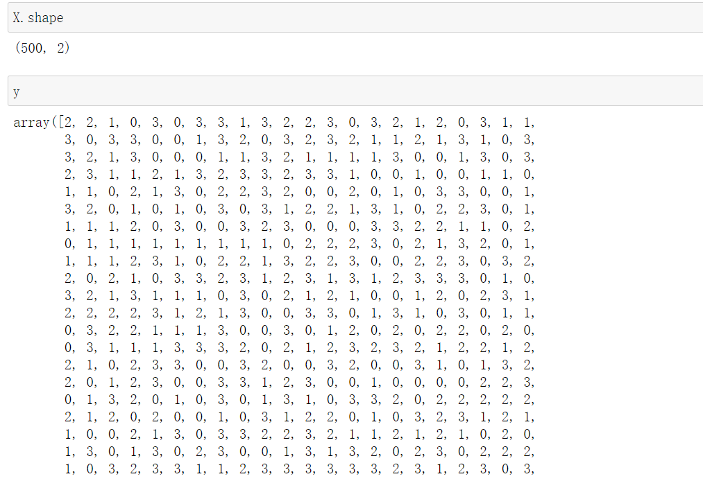
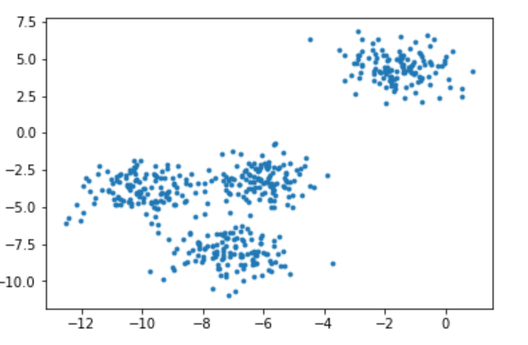
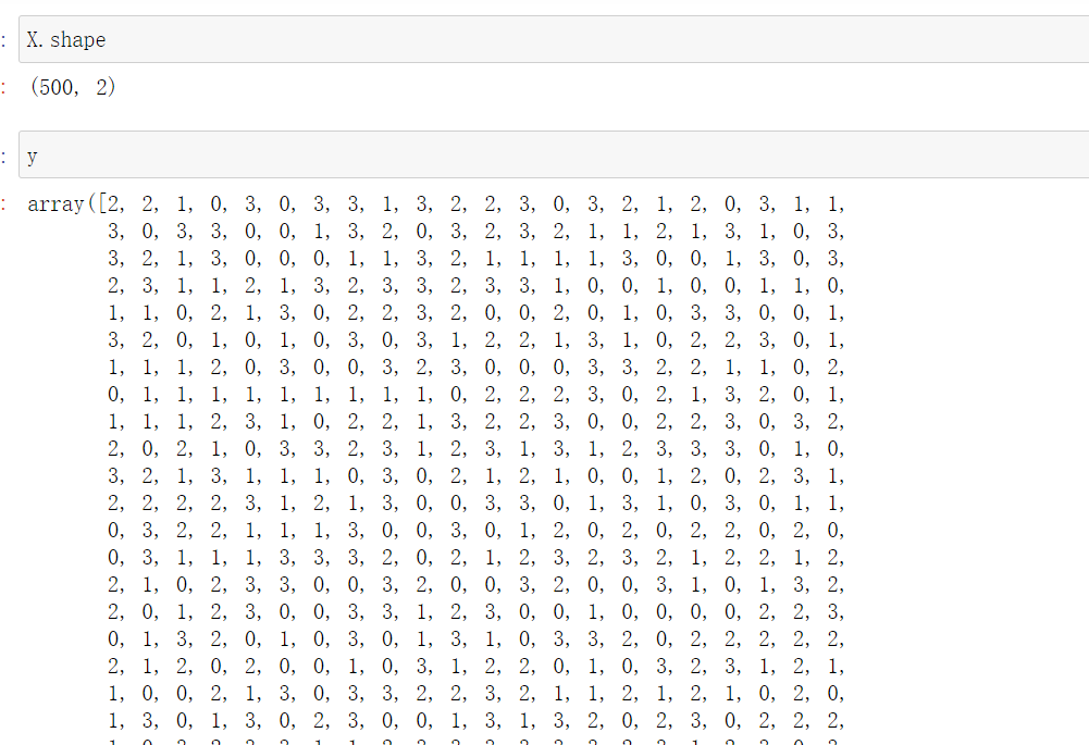
First, let's create a dataset ourselves. Such data sets are created by ourselves, so they are labeled (99% of the data normally obtained will not have labels).
2.1.1.1 import package and create dataset
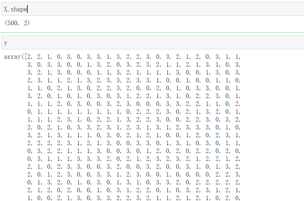
from sklearn.datasets import make_blobs #Create dataset
import matplotlib.pyplot as plt

#500 pieces of data, each data has 2 features and 4 centroids, that is, it is divided into 4 clusters and set random parameters
X,y = make_blobs(n_samples=500,n_features=2,centers=4,random_state=1)
2.1.1.2 draw the data distribution with and without color of the sample respectively
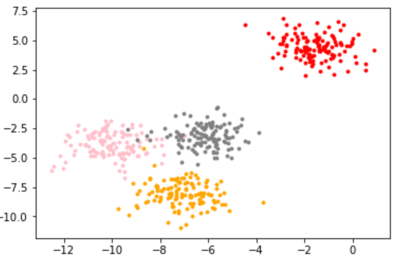
Because the dataset is created by ourselves, there are labels, that is, the dataset has been divided. Here, the colored graph is the distribution of labels created by sklearn. Here, we print out the colored and not low colored ones for observation
fig,axl = plt.subplots(1)

axl.scatter(X[:,0],X[:,1]
            ,marker='o' #Shape of point
            ,s=8#Point size
           )
plt.show()
color = ['red','pink','orange','gray']
fig,axl = plt.subplots(1)

for i in range(4):
    axl.scatter(X[y==i,0],X[y==i,1]
               ,marker='o'
               ,s=8
               ,color=color[i]
               )

plt.show()
2.1.1.3 KMeans clustering based on this distribution
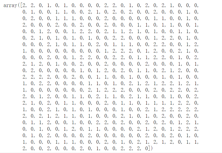
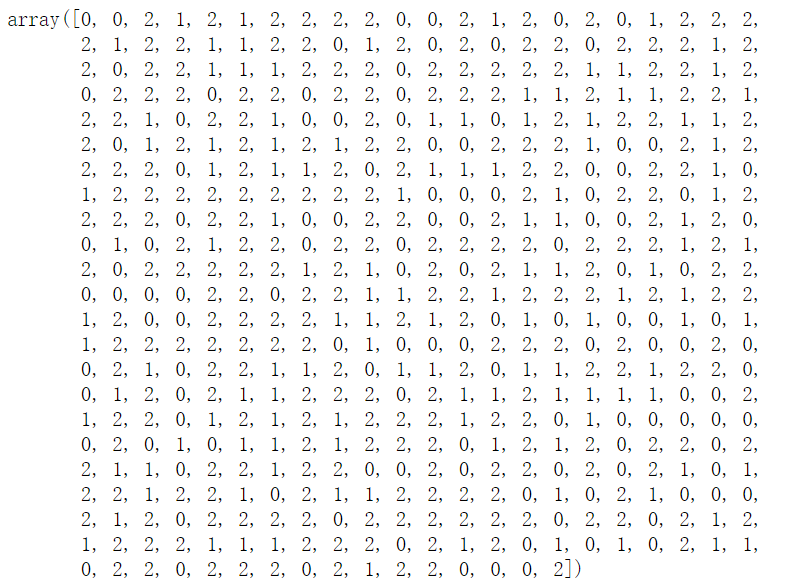
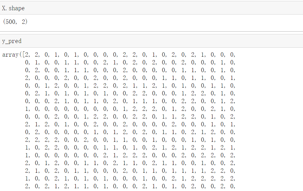
from sklearn.cluster import KMeans #KMeans

#According to the above distribution diagram, it is assumed to be divided into 3 clusters
n_clusters = 3
cluster = KMeans(n_clusters=n_clusters,random_state=0).fit(X)

#Important attribute labels_, View the clustered categories and the corresponding classes of each sample
y_pred = cluster.labels_
y_pred

#KMeans do not need to build models or predict results, so we only need fit to get clustering results
#KMeans also have interfaces predict and fit_predict, which means learning data X and predicting the class of X
#But the result is the first mock exam of the property labels after we call predict directly, and then we call fit.
pre = cluster.fit_predict(X)
pre
#The results obtained by using labels and predict are the same
pre == y_pred
2.1.1.4 when does kmeans use labels and predict
When the amount of data is too large, we need to predict. In fact, we don't need to use all the data to find the centroid. A small amount of data can help us determine the centroid. When the amount of data is very large, we can use part of the data to help us confirm the clustering results of the remaining data of the centroid, and use predict to call
#Assuming that the data is very large, select 250 data for training
cluster_smallsub = KMeans(n_clusters=n_clusters, random_state=0).fit(X[:250])
#Use predict
y_pred_ = cluster_smallsub.predict(X)
y_pred_
When the amount of data is very large, the effect will be good
However, such a result obtained from the operation will certainly be inconsistent with all the data of direct fit. Sometimes, when we don't require such precision, or our data volume is too large, we can use this method and use the interface predict
If the amount of data is OK, it is not very large. After using fit directly, the property.labels_ is called. Bring it up
#It can be seen that the results obtained are different from all x of fit
y_pred == y_pred_
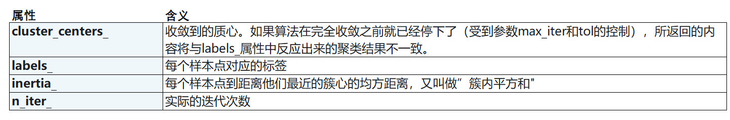
2.1.1.5 important attribute cluster_centers_, View centroid
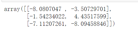
#Important attribute cLuster_centers_, View centroid
centroid = cluster.cluster_centers_
centroid
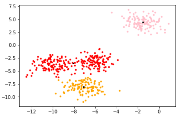
Three centroids are obtained, and the number of each group is the corresponding coordinate
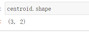
centroid.shape
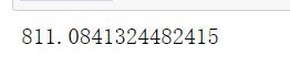
2.1.1.6 important attributes inertia#, View sum of squares of total distances
#Important attribute inertia_, View sum of squares of total distances
inertia = cluster.inertia_
inertia
2.1.1.7 draw the image after KMeans clustering
color = ["red","pink","orange","gray"]
fig,axl = plt.subplots(1)

#n_clusters is defined as 3 at the beginning
for i in range(n_clusters):
    axl.scatter(X[y_pred==i,0],X[y_pred==i,1]
               ,marker='o'
               ,s=8
               ,c=color[i]
               )

 #Draw the center of mass
axl.scatter(centroid[:,0],centroid[:,1]
           ,marker='x'
           ,s=8
           ,c='black')
plt.show()
2.1.1.8 look at the difference n_ Performance of kmean under clusters
- Equal to 4
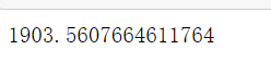
#What would happen to Inertia if we changed our guess to 4?
n_clusters = 4
cluster_ = KMeans(n_clusters=n_clusters, random_state=0).fit(X)
#Sum of squares of total distances
inertia_ = cluster_.inertia_
inertia_
- Equal to 5
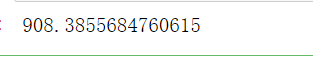
n_clusters = 5
cluster_ = KMeans(n_clusters=n_clusters, random_state=0).fit(X)
inertia_ = cluster_.inertia_
inertia_
- When it's 500
n_clusters = 500
cluster_ = KMeans(n_clusters=n_clusters, random_state=0).fit(X)
inertia_ = cluster_.inertia_
inertia_

As you can see, with n_ With the increase of clusters, it is found that the sum of squares of the total distance decreases when n_ When clusters is 500, the sum of squares of the total distance is 0, because the sum of squares of the total distance is obtained from other samples in the same cluster, so it will increase with n_ The larger the clusters, the smaller they are. We can't use n_clusters as the evaluation criteria. The corresponding model evaluation criteria will be introduced below
2.1.2 model evaluation index of clustering algorithm
Different from classification model and regression, model evaluation of clustering algorithm is not a simple thing. In the classification, there are direct results (labels) output, and the classification results can be divided into right and wrong, so we use the prediction accuracy, confusion matrix, ROC curve and other indicators to evaluate, but in any case, we find the correct answer in the "model" In regression, we have SSE mean square error and loss function to measure the fitting degree of the model due to fitting data, but these indicators can not be used in clustering.
The result of clustering model is not a label output, and the clustering result is uncertain. Its quality is determined by business requirements or algorithm requirements, and there is no always correct answer.
How to measure the effect of clustering
KMeans aims to ensure that "intra cluster differences are small, while intra cluster differences are large", so we can measure the effect of clustering by measuring intra cluster differences. As mentioned earlier, Inertia is an indicator to measure intra cluster differences. The smaller the Inertia, the better the model. Therefore, can we use Inertia as a clustering indicator?
-
Yes, but the shortcomings and limits of this indicator are too large.
-
It is not bounded. We only know that the smaller the Inertia, the better, and 0 is the best, but we don't know whether a smaller Inertia has reached the limit of the model or whether it can continue to improve.
-
Its calculation is too vulnerable to the number of features. When the data dimension is large, the calculation amount of Inertia will fall into the curse of dimension, and the calculation amount will explode, which is not suitable for evaluating the model again and again.
-
It will be affected by the super parameter K (n_clusters). In our previous common sense, we have found that with the increase of K, Inertia is bound to become smaller and smaller, but this does not mean that the effect of the model is getting better and better
-
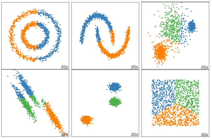
Inertia assumes the distribution of data. It assumes that the data satisfies a convex distribution (that is, the data looks like a convex function on a two-dimensional plane image), and it assumes that the data is isotropic, that is, the attributes of the data represent the same meaning in different directions. But this is often not the case with real data. Therefore, using inertia as the evaluation index will make the clustering algorithm perform poorly in some slender clusters, ring clusters, or irregular manifolds:
2.1.2.1 when the real label is known (it will not happen in the real situation)
Although we do not input real labels in the clustering, it does not mean that the data we have must not have real labels or there must be no reference information. Of course, in reality, it is very rare (almost impossible) to have a real label. If we have real labels, we prefer to use classification algorithms. However, it does not rule out the possibility that we may still use clustering algorithm. If we have real clustering data of samples, we can measure the effect of clustering for the results of clustering algorithm and real results. There are three common methods:
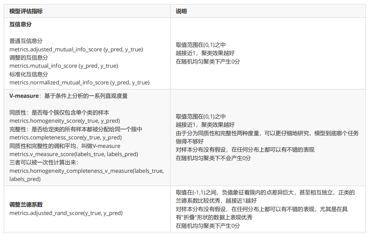
The common point of the three methods is that the higher the score, the better the effect. Put the label clustered by kmeans and the original label to obtain the corresponding score for evaluation
2.1.2.2 when the real label is unknown: contour coefficient
In 99% of cases, we are exploring the data without real labels, that is, clustering the data without real answers. Such clustering completely depends on the evaluation of the density within the cluster (small difference within the cluster) and the dispersion between clusters (large difference outside the cluster) to evaluate the effect of clustering. The contour coefficient is the most commonly used evaluation index of clustering algorithm. It is defined for each sample and can measure:
- The similarity a between the sample and other samples in its own cluster is equal to the average distance between the sample and all other points in the same cluster
- The similarity b between the sample and the sample in other clusters is equal to the average distance between the sample and all points in the next nearest cluster
According to the requirements of clustering, "the difference within the cluster is small and the difference outside the cluster is large", we hope that b will always be greater than a, and the greater the better.
The contour coefficient of a single sample is calculated as:
s
=
b
−
a
max
(
a
,
b
)
s=\frac{b-a}{\max(a,b)}
s=max(a,b)b−a
This formula can be resolved as:
f
(
n
)
=
{
1
−
a
/
b
,
if
a
<
b
0
,
if
a
=
b
b
/
a
−
1
if
a
>
b
f(n)= \begin{cases} 1-a/b, & \text {if $a<b$} \\ 0, & \text{if $a=b$} \\ b/a-1 & \text{if $a>b$} \end{cases}
f(n)=⎩⎪⎨⎪⎧1−a/b,0,b/a−1if a<bif a=bif a>b
It is easy to understand that the contour coefficient range is (- 1,1)
- The closer the value is to 1, it means that the sample is very similar to the sample in its own cluster and is not similar to the sample in other clusters.
- When the sample points are more similar to the samples outside the cluster, the contour coefficient is negative.
- When the contour coefficient is 0, it means that the sample similarity in the two clusters is the same, and the two clusters should be one cluster.
If most samples in a cluster have relatively high contour coefficients, the cluster will have higher total contour coefficients, and the higher the average contour coefficient of the whole data set, the clustering is appropriate. If many sample points have low contour coefficients or even negative values, the clustering is inappropriate, and the super parameter K of clustering may be set too large or too small.
In sklearn:
- The class silhouette_score in the module metrics is used to calculate the contour coefficient. It returns the mean value of the contour coefficient of all samples in a data set.
- In the silhouette_sample in the metrics module, its parameters are consistent with the contour coefficient, but it returns the contour coefficient of each sample in the dataset.
Let's see how the contour coefficient performs on the data set we built above:
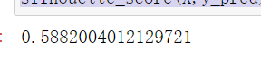
from sklearn.metrics import silhouette_score #Mean value of contour coefficient of all samples
from sklearn.metrics import silhouette_samples #Each sample has its own contour coefficient

#y_pred is derived from the above. labels
silhouette_score(X,y_pred)
#Returns the contour coefficient for each sample
silhouette_samples(X,y_pred).shape
#500 are returned, that is, a contour coefficient is calculated for each sample

Let's see how n_clusters behave when they grow
#Run the above cluster divided into 4 clusters_
silhouette_score(X,cluster_.labels_)
#After running the above cluster_divided into 5 clusters, it is found that it decreases, indicating that this does not increase with the increase of n_clusters
silhouette_score(X,cluster_.labels_)
It can be observed that when 4 is taken, the effect is better, and when 5 is taken, the effect becomes worse
Contour coefficient has many advantages. It takes value in limited space, which makes us have a "reference" for the clustering effect of the model Moreover, the contour coefficient does not assume the distribution of data, so it performs well on many data sets. However, it performs best when each cluster is segmented and cleaned. However, the contour coefficient also has defects, and its performance will be falsely high on convex classes, such as clustering based on density or clustering results obtained through DBSCAN. If the contour coefficient is used to measure it, it will be better It shows a higher score than the real clustering effect.
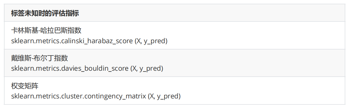
2.1.2.3 when the real label is unknown: calinski harabaz index
In addition to the most commonly used contour coefficient, we also have the calinski harabaz index (CHI, also known as variance ratio standard), Davies bouldin index and Contingency Matrix.
Let's focus on the karinski harabaz index. The higher the calinski harabaz index, the better. For clusters with K clusters, the calinski harabaz index s(k) is written as follows:
s
(
k
)
=
T
r
(
B
k
)
T
r
(
W
k
)
∗
N
−
k
k
−
1
s(k)=\frac{Tr(B_k)}{Tr(W_k)}*\frac{N-k}{k-1}
s(k)=Tr(Wk)Tr(Bk)∗k−1N−k
- N : N: N: Sample size in dataset
- k : k: k: Number of clusters (i.e. number of categories)
- B k : B_k: Bk: inter group discrete matrix, i.e. covariance matrix between different clusters
- W k : W_k: Wk: intra cluster discrete matrix, that is, the covariance matrix of data in a cluster
- T r : Tr: Tr: trace of matrix. In linear algebra, an n × N the sum of the elements on the main diagonal of matrix A (the diagonal from the upper left to the lower right) is called the trace (or trace number) of matrix A, which is generally recorded as T r ( A ) Tr(A) Tr(A).
The higher the degree of dispersion between the data, the larger the trace of the covariance matrix.
The lower the dispersion in the group, the smaller the trace of covariance, T r ( W k ) Tr(W_k) The smaller Tr(Wk), the greater the degree of dispersion between groups, and the greater the trace of covariance, T r ( B k ) Tr(B_k) The larger Tr(Bk) is, which is exactly what we want. Therefore, the higher the calinski harabaz index, the better.
from sklearn.metrics import calinski_harabasz_score #CHI

#Clustering after KMeans training in y_pred
calinski_harabasz_score(X, y_pred)
Although the calinski harabaz index is unbounded, clustering on convex data will also show virtual heights. However, compared with the contour coefficient, it has a great advantage that the calculation is very fast. Previously, we used the magic command%% timeit to calculate the operation time of a command. Today, we choose another method: timestamp to calculate the running time.
from time import time

#Run time using CHI
t0 = time()
calinski_harabasz_score(X, y_pred)
time() - t0
> 0.000997304916381836

#Run time using profile factor
t0 = time()
silhouette_score(X,y_pred)
time() - t0
> 0.00795125961303711

#Convert timestamp to time
import datetime
datetime.datetime.fromtimestamp(t0).strftime("%Y-%m-%d %H:%M:%S")
>'2021-11-18 21:34:00'

#The running time is about 7 times
0.00795125961303711//0.000997304916381836=7.0
2.1.3 case: select n_clusters based on contour coefficient
We usually draw the contour coefficient distribution map and the data distribution map after clustering to select our best n_clusters.
1. Import library
from sklearn.cluster import KMeans #KMeans clustering algorithm
from sklearn.metrics import silhouette_samples, silhouette_score #The contour coefficient of each sample and the average contour coefficient of all samples
import matplotlib.pyplot as plt
import matplotlib.cm as cm #colormap can use a specific decimal to represent a color
import numpy as np
import pandas as pd
2. Set canvas
Find the best n based on the contour coefficient_ clusters
Know the contour coefficient of each aggregated class, and compare it with that of each class
Know the distribution after clustering
#First set the number of clusters we want to divide
n_clusters = 4

#Create a canvas with one row and two columns
fig, (ax1,ax2) = plt.subplots(1,2)

#Set the canvas size, that is, the width of both palettes is 9 and the height is 7
fig.set_size_inches(18,7)

#The first graph is the contour coefficient image, which is a horizontal bar graph composed of the contour coefficients of each cluster
#The abscissa of the horizontal bar graph is the value of the contour coefficient, and the ordinate is the sample

#First, set the abscissa
#The value of contour coefficient is (- 1,1), but we hope that the contour coefficient is greater than 0. If it is less than 0, the proof score is not good
#Too long abscissa is not conducive to visualization, so (- 0.1, 1) is taken as the range
ax1.set_xlim([-0.1,1])


#For the ordinate, starting from 0, the maximum value is X.shape[0], which is the number of samples
#We put the of each cluster together, and there are gaps between different clusters
#When setting the range of ordinates, add a distance (n_clusters+1) * 10 to X.shape[0] as the interval
#The reason for + 1 here is that the drawing should not only have a gap between columns, but also have a gap with the x-axis and the top
ax1.set_ylim([0, X.shape[0]+(n_clusters + 1)*10])
3. Preparation of data for modeling and drawing
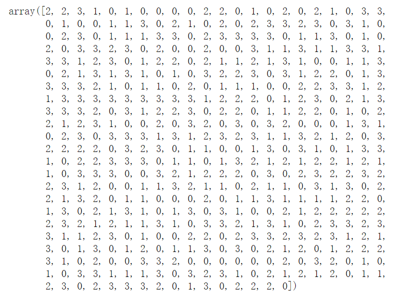
#Start modeling and view the clustered tags
clusterer = KMeans(n_clusters=n_clusters,random_state=10).fit(X)
clusterer_labels = clusterer.labels_
#Clustering good results
clusterer_labels
#Call contour coefficient score, silhouette_score is the mean value of the contour coefficient of the total sample
#What you need to input is the characteristic matrix X and the label after clustering
silhouette_avg = silhouette_score(X,clusterer_labels)

#Print in different N_ Under clusters, the overall contour coefficient
print(f'n_clusters The value of is{n_clusters},   The average contour coefficient of the whole sample is{silhouette_avg}')

#silhouette_samples returns the contour coefficient of each sample as the value of the x-axis
sample_silhouette_values = silhouette_samples(X,clusterer_labels)
sample_silhouette_values.shape

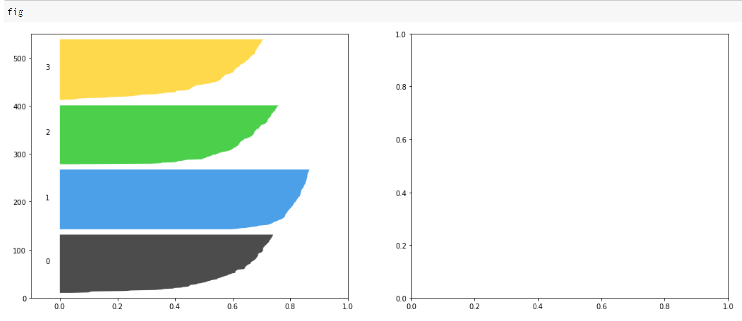
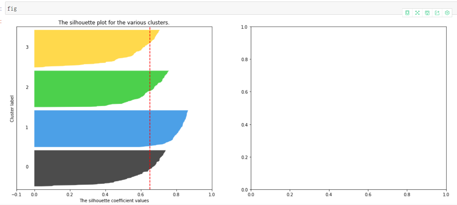
4. Draw sub Figure 1 and look at the histogram of clustering contour coefficient
#Set an initial value of the y-axis, because you don't want the drawn image to be pasted on the x-axis, keep some distance from the x-axis
y_lower = 10

#Next, cycle through each cluster
for i in range(n_clusters):
    #The contour coefficients belonging to cluster i are extracted from the contour coefficients of each sample obtained, and they need to be sorted
    #Because the sorted image looks like increasing or decreasing, it can be observed more intuitively
    #sample_silhouette_values is the contour coefficient, cluster_ Labels is the clustering of each sample, cluster_ Labels = = i is the contour coefficient of cluster i
    ith_cluster_silhouette_values = sample_silhouette_values[clusterer_labels == i]

    #Will change the order of the original data
    ith_cluster_silhouette_values.sort()

    #What is the number of samples in this cluster
    size_cluster_i = ith_cluster_silhouette_values.shape[0]

    #The value of this cluster on the y-axis should be from y_lower is taken as the minimum value from the beginning and the number of samples in this cluster is taken as the end value
    y_upper = y_lower + size_cluster_i

    #In the colormap library, use decimals to call colors
    #In nipy_spectral([enter any decimal to represent a color])
    #The hope here is that the color of each cluster is different, and the required color type is the number of clusters
    #Using this can ensure that different clusters have different colors. As long as the decimal is determined, the color will not change
    #Not necessarily this division, as long as it is guaranteed to be decimal and the decimal of the same cluster is the same
    color = cm.nipy_spectral(float(i)/n_clusters)

    #Start filling the contents of sub Figure 1
    #fill_between is a function that makes the histogram in a range display the same color
    #fill_ The range of betweenx is on the ordinate
    #fill_ The range of between is on the abscissa
    #fill_betweenx parameters should be entered (lower limit of ordinate, upper limit of ordinate, value of corresponding abscissa, color of histogram)
    ax1.fill_betweenx(np.arange(y_lower,y_upper)
                     ,ith_cluster_silhouette_values
                     ,facecolor=color
                     ,alpha=0.7)

    #Write a number for the contour coefficient of each cluster and let the number display in the middle of each bar graph on the coordinate axis
    #The parameters of text are (abscissa of the position where the number is to be displayed, ordinate of the position where the number is to be displayed, and number content to be displayed)
    ax1.text(-0.05 #In order not to display at the position of 0, it is -0.05, so it can be empty
            ,y_lower + 0.5*size_cluster_i #Get the middle value of the number of samples of a cluster as the storage location of the number
            ,str(i))

    #Calculate the initial value above the new Y-axis for the next cluster, which is the upper limit of y plus 10 after each iteration
    #This ensures that the next cluster will not cover the last cluster, and there are gaps between different clusters
    #The price here is 10 because the initial value of y set at the top is 10, which means that each gap is 10
    y_lower = y_upper + 10
#Set the title, x-axis name and y-axis name for sub Figure 1
ax1.set_title("The silhouette plot for the various clusters.")
ax1.set_xlabel("The silhouette coefficient values")
ax1.set_ylabel("Cluster label")

#Draw the average contour coefficient of the total sample in the subgraph with a dotted line for comparison
ax1.axvline(x=silhouette_avg, color="red", linestyle="--")

#Set the y-axis not to display the scale
ax1.set_yticks([])

#Sets the value range of the x-axis
ax1.set_xticks([-0.1, 0, 0.2, 0.4, 0.6, 0.8, 1])
5. Draw sub Figure 2, scatter distribution diagram and centroid of each sample
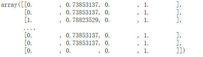
#To process the second sub graph, first obtain the color. The color here should be the same as the color corresponding to each cluster when drawing the sub graph above, which is the reason for using the colormap
#Therefore, the calculation method of the decimal corresponding to the color should be the same as when drawing sub Figure 1
#Therefore, the initial clustering result is converted to float for calculation
colors = cm.nipy_spectral(clusterer_labels.astype(float) / n_clusters)
colors
Each number represents a color map
#Draw a scatter diagram, as in the first clustering above
ax2.scatter(X[:,0],X[:,1]
,marker='o'
,s=8
,c=colors)
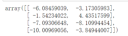
#Get the centroid in each cluster
centers = clusterer.cluster_centers_
centers
centroid
#Add centroid to scatter plot
ax2.scatter(centers[:,0],centers[:,1]
           ,marker='x'
           ,s=200
           ,c='red'
           ,alpha=1)

#Set the title for sub Figure 2
ax2.set_title("The visualization of the clustered data.")
ax2.set_xlabel("Feature space for the 1st feature")
ax2.set_ylabel("Feature space for the 2nd feature")

#Set the general title of fig
fig.suptitle(("Silhouette analysis for KMeans clustering on sample data"
              "with n_clusters = %d" % n_clusters),
             fontsize=14, fontweight='bold'#Use bold
            )

plt.show()
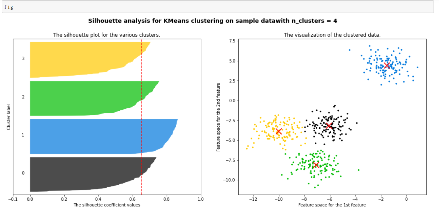
It can be seen that the blue cluster is the best. Basically, all of them have passed the average line. Generally speaking, it is good. Some of each cluster have passed the average line
All contribute to the contour coefficient. Those less than the average can be regarded as a drag, which is very good for this kind of clustering
6. Draw a graph for different cluster numbers to select n_clusters (although there are many comments on the above steps, many of them are the same as those above, which is helpful for understanding here)
from sklearn.cluster import KMeans
from sklearn.metrics import silhouette_samples, silhouette_score

import matplotlib.pyplot as plt
import matplotlib.cm as cm
import numpy as np

for n_clusters in [2,3,4,5,6,7]:
    #First set the number of clusters we want to divide
    n_clusters = n_clusters

    #Create a canvas with one row and two columns
    fig, (ax1,ax2) = plt.subplots(1,2)

    #Set the canvas size, that is, the width of both palettes is 9 and the height is 7
    fig.set_size_inches(18,7)

    #The first graph is the contour coefficient image, which is a horizontal bar graph composed of the contour coefficients of each cluster
    #The abscissa of the horizontal bar graph is the value of the contour coefficient, and the ordinate is the sample

    #First, set the abscissa
    #The value of contour coefficient is (- 1,1), but we hope that the contour coefficient is greater than 0. If it is less than 0, the proof score is not good
    #Too long abscissa is not conducive to visualization, so (- 0.1, 1) is taken as the range
    ax1.set_xlim([-0.1,1])


    #For the ordinate, starting from 0, the maximum value is X.shape[0], which is the number of samples
    #We put the of each cluster together, and there are gaps between different clusters
    #When setting the range of ordinates, add a distance (n_clusters+1) * 10 to X.shape[0] as the interval
    ax1.set_ylim([0, X.shape[0]+(n_clusters + 1)*10])

    #Start modeling and view the clustered tags
    clusterer = KMeans(n_clusters=n_clusters, random_state=10).fit(X)
    cluster_labels = clusterer.labels_

    #Call contour coefficient score, silhouette_score is the mean value of the contour coefficient of the total sample
    #What you need to input is the characteristic matrix X and the label after clustering
    silhouette_avg = silhouette_score(X, cluster_labels)

    #Print in different N_ Under clusters, the overall contour coefficient
    print(f'n_clusters The value of is{n_clusters},   The average contour coefficient of the whole sample is{silhouette_avg}')

    #silhouette_samples returns the contour coefficient of each sample as the value of the x-axis
    sample_silhouette_values = silhouette_samples(X, cluster_labels)


    #Set an initial value of the y-axis, because you don't want the drawn image to be pasted on the x-axis, keep some distance from the x-axis
    y_lower = 10

    #Next, cycle through each cluster
    for i in range(n_clusters):
        #The contour coefficients belonging to cluster i are extracted from the contour coefficients of each sample obtained, and they need to be sorted
        #Because the sorted image looks like increasing or decreasing, it can be observed more intuitively
        #sample_silhouette_values is the contour coefficient, cluster_ Labels is the clustering of each sample, cluster_ Labels = = i is the contour coefficient of cluster i
        ith_cluster_silhouette_values = sample_silhouette_values[clusterer_labels == i]

        #Will change the order of the original data
        ith_cluster_silhouette_values.sort()

        #What is the number of samples in this cluster
        size_cluster_i = ith_cluster_silhouette_values.shape[0]

        #The value of this cluster on the y-axis should be from y_lower is taken as the minimum value from the beginning and the number of samples in this cluster is taken as the end value
        y_upper = y_lower + size_cluster_i

        #In the colormap library, use decimals to call colors
        #In nipy_spectral([enter any decimal to represent a color])
        #The hope here is that the color of each cluster is different, and the required color type is the number of clusters
        #Using this can ensure that different clusters have different colors. As long as the decimal is determined, the color will not change
        #Not necessarily this division, as long as it is guaranteed to be decimal and the decimal of the same cluster is the same
        color = cm.nipy_spectral(float(i)/n_clusters)

        #Start filling the contents of sub Figure 1
        #fill_between is a function that makes the histogram in a range display the same color
        #fill_ The range of betweenx is on the ordinate
        #fill_ The range of between is on the abscissa
        #fill_betweenx parameters should be entered (lower limit of ordinate, upper limit of ordinate, value of corresponding abscissa, color of histogram)
        ax1.fill_betweenx(np.arange(y_lower,y_upper)
                         ,ith_cluster_silhouette_values
                         ,facecolor=color
                         ,alpha=0.7)

        #Write a number for the contour coefficient of each cluster and let the number display in the middle of each bar graph on the coordinate axis
        #The parameters of text are (abscissa of the position where the number is to be displayed, ordinate of the position where the number is to be displayed, and number content to be displayed)
        ax1.text(-0.05 #In order not to display at the position of 0, it is -0.05, so it can be empty
                ,y_lower + 0.5*size_cluster_i #Get the middle value of the number of samples of a cluster as the storage location of the number
                ,str(i))

        #Calculate the initial value above the new Y-axis for the next cluster, which is the upper limit of y plus 10 after each iteration
        #This ensures that the next cluster will not cover the last cluster, and there are gaps between different clusters
        #The price here is 10 because the initial value of y set at the top is 10, which means that each gap is 10
        y_lower = y_upper + 10

    #Set the title, x-axis name and y-axis name for sub Figure 1
    ax1.set_title("The silhouette plot for the various clusters.")
    ax1.set_xlabel("The silhouette coefficient values")
    ax1.set_ylabel("Cluster label")

    #Draw the average contour coefficient of the total sample in the subgraph with a dotted line for comparison
    ax1.axvline(x=silhouette_avg, color="red", linestyle="--")

    #Set the y-axis not to display the scale
    ax1.set_yticks([])

    #Sets the value range of the x-axis
    ax1.set_xticks([-0.1, 0, 0.2, 0.4, 0.6, 0.8, 1])

    #To process the second sub graph, first obtain the color. The color here should be the same as the color corresponding to each cluster when drawing the sub graph above, which is the reason for using the colormap
    #Therefore, the calculation method of the decimal corresponding to the color should be the same as when drawing sub Figure 1
    #Therefore, the initial clustering result is converted to float for calculation
    colors = cm.nipy_spectral(cluster_labels.astype(float) / n_clusters)

    #Draw a scatter diagram, as in the first clustering above
    ax2.scatter(X[:,0],X[:,1]
               ,marker='o'
               ,s=8
               ,c=colors)

    #Get the centroid in each cluster
    centers = clusterer.cluster_centers_

    #Add centroid to scatter plot
    ax2.scatter(centers[:, 0], centers[:, 1], marker='x',
                c="red", alpha=1, s=200)

    #Set the title for sub Figure 2
    ax2.set_title("The visualization of the clustered data.")
    ax2.set_xlabel("Feature space for the 1st feature")
    ax2.set_ylabel("Feature space for the 2nd feature")

    #Set the general title of fig
    fig.suptitle(("Silhouette analysis for KMeans clustering on sample data"
                  "with n_clusters = %d" % n_clusters),
                 fontsize=14, fontweight='bold'#Use bold
                )

    plt.show()
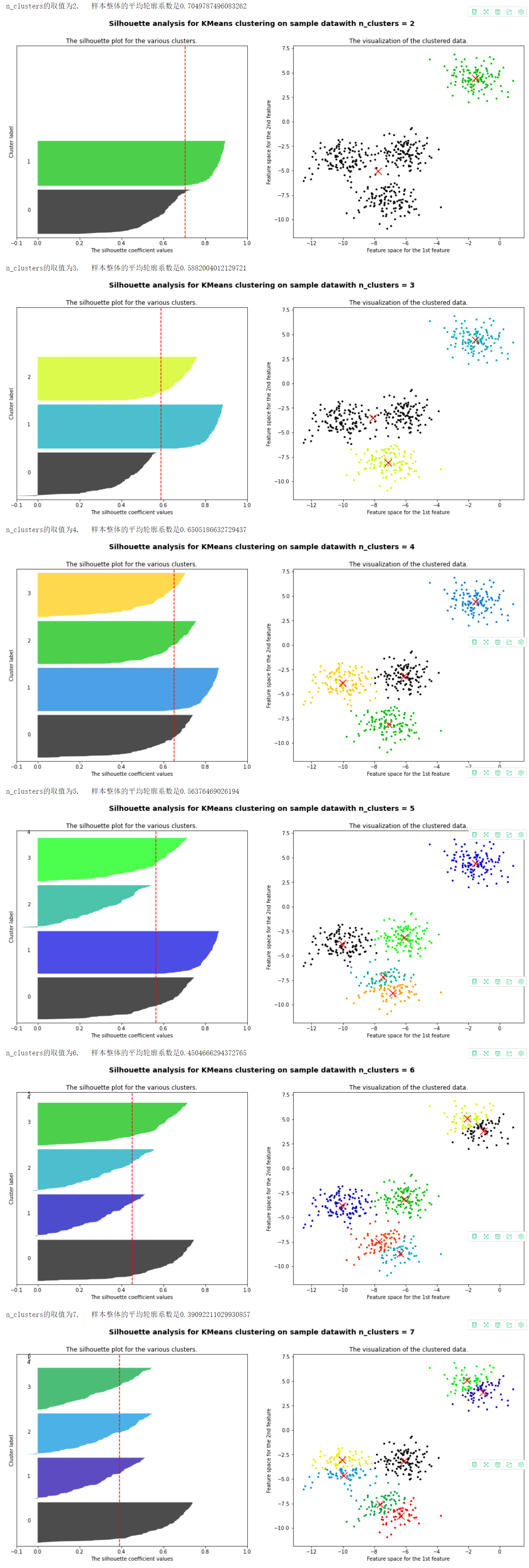
7. Summarize according to the figure above
- It can be seen that when the cluster is divided into 2 clusters, the green ones score well, but the black ones pull down the mean value, and the contour coefficient is 0.7. For analysis, such scoring is not impossible, mainly depending on the specific requirements
- When dividing into three clusters, it can be seen that the black ones do not exceed the average contour coefficient, and some contour coefficients are less than 0, so this method is not good
- When divided into 4 clusters, the effect is still very good, and each cluster contributes to the average contour coefficient
- When 5 clusters are divided, it is found that two clusters lower the average contour coefficient, and there is a contour coefficient less than 0
- When there are more and more clusters, there are more and more clusters with smaller and smaller contribution, and even those with contour coefficient less than 0, which proves that these methods are very bad
After screening, it can be seen that when it is divided into 2 clusters or 4 clusters, the effect is still very good, and the corresponding selection can be made according to the actual situation
2.2 important parameters init & random_ state & n_ Init: how to place the initial centroid?
An important step in K-means is to place the initial centroid. If there is enough time, K-means will converge, but Inertia may converge to the local minimum. Whether it can converge to the real minimum depends largely on the initialization of the centroid. init is a parameter used to help us decide how to initialize.
If the initial centroid is placed at different positions, the clustering results are likely to be different. A good centroid selection can make K-Means avoid more calculations and make the convergence of the algorithm stable and faster. When we explained the placement of the initial centroid, we used the "random" method to extract k samples from the sample points as the initial centroid. This method obviously does not conform to the "stable and faster" principle "For this purpose, we can use the random_state parameter to control that the initial centroid generated each time is in the same position, and even draw a learning curve to determine which integer the optimal random_state is (not often used).
A random_state corresponds to a random number seed randomly initialized by the centroid. If the random number seed is not specified, the K-means in sklearn will not only select a random mode to throw the result, but will run multiple times under each random number seed, and use the random number seed with the best result as the initial centroid. We can use the parameter n_init to select each random number seed The number of times to run under the machine number seed. This parameter is not commonly used. It defaults to 10 times. If we want to run the results more accurately, we can increase the value of this parameter n_init to increase the number of times to run under each random number seed.
In order to optimize the method of selecting initial centroids, Arthur, David, and Sergei Vassilvitskii developed the "k-means + +" initialization scheme in 2007, which makes the initial centroids (usually) far away from each other, so as to guide more reliable results than random initialization.
In sklearn, we use the parameter init ='k-means + +' to select the scheme using k-means + + as the centroid initialization. Generally speaking, it is recommended to keep the default "K-means + +" method.
- init: you can enter "K-means + +," random "or an n-dimensional array. This is the method to initialize the centroid. The default is "K-means + +". Enter "K-means + +": a smart way to select the initial cluster center for k-means clustering to accelerate convergence. If an n-dimensional array is entered, the shape of the array should be (n_clusters, n_features) and give the initial centroid.
- random_state: controls the random number seed of each centroid random initialization
- n_init: integer, default 10, the number of times to run k-means algorithm using seeds randomly initialized with different centroids. The final result will be calculated based on Inertia n_ Optimal output after init consecutive runs
plus = KMeans(n_clusters = 10).fit(X)
#Number of iterations
plus.n_iter_
>7

random = KMeans(n_clusters = 10,init="random",random_state=420).fit(X)
#Number of iterations
random.n_iter_
>19
It can be seen that using the default init = 'k-means + +' has fewer iterations than random. This is random and may be very close, but it will not be larger than random.
However, the running time of k-means + + is longer than that of random. The preliminary guess is that the calculation is complex. If you want to understand it in detail, look at the source code
2.3 important parameters Max_ ITER & tol: stop the iteration
When describing the basic flow of K-Means, we mentioned that when the centroid no longer moves, the Kmeans algorithm will stop. But before full convergence, we can also use max_iter, the maximum number of iterations, or tol, the amount of Inertia decrease between two iterations. These two parameters are used to stop the iteration in advance. Sometimes, when our n_ The clusters selection does not conform to the natural distribution of the data, or we must fill in the n that does not conform to the natural distribution of the data for business needs_ Clusters, stopping the iteration in advance can improve the performance of the model.
- max_iter: integer, 300 by default, the maximum number of iterations of k-means algorithm in a single run
- TOL: floating point number. The default is 1e-4. The amount of Inertia falling between two iterations. If the value of Inertia falling between two iterations is less than the value set by tol, the iteration will stop
random = KMeans(n_clusters = 10,init="random",max_iter=10,random_state=420).fit(X)
y_pred_max10 = random.labels_
silhouette_score(X,y_pred_max10)
>0.3952586444034157

random = KMeans(n_clusters = 10,init="random",max_iter=20,random_state=420).fit(X)
y_pred_max20 = random.labels_
silhouette_score(X,y_pred_max20)
>0.3401504537571701
You can see the setting max_iter equal to 10 performs better than ITER equal to 20. Here is to understand this parameter, so let n_clusters = 10
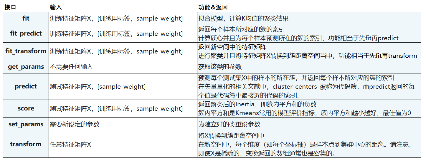
2.4 important attributes and interfaces
2.5 function cluster.k_means
sklearn.cluster.k_means (X, n_clusters, sample_weight=None, init='k-means++', precompute_distances='auto',n_init=10, max_iter=300, verbose=False, tol=0.0001, random_state=None, copy_x=True, n_jobs=None,algorithm='auto', return_n_iter=False)
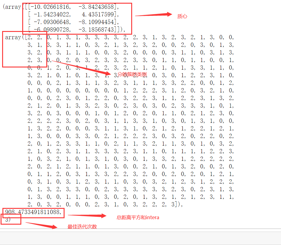
Function K_ The use of means is actually very similar to that of a class, but a function inputs a series of values and returns the result directly. Once, function k_means will return the centroid, the label of the cluster corresponding to each sample, inertia and the optimal number of iterations in turn.
from sklearn.cluster import k_means

#Enter the characteristic matrix and the number of clusters to be divided, return_n_iter defaults to False. If it is adjusted to True, the maximum number of iterations can be returned
k_means(X,4,return_n_iter=True)
summary
KMeans is the simplest clustering algorithm, but it has a lot of code and needs a little patience