sample
Positive samples: samples belonging to a certain class (generally the desired class). In this case is a passing student.
Negative samples: samples that do not belong to this category. In this case, it is a failed student.
  y_pred = [0, 0, 0, 0, 0, 0, 1, 1, 1, 1]
  y_true = [0, 0, 0, 0, 1, 1, 1, 1, 0, 0]
The above 0 represents failure and 1 represents passing. The positive sample here represents passing.
TP,FP,FN,TN
| Positive class | Negative class | |
|---|---|---|
| Retrieved | True Positive | False Positive |
| Not retrieved | False Negative | True Negative |
- TP: the retrieved positive sample is actually a positive sample (correctly identified)
In this case, the performance is: pass the prediction and pass the practice. This example TP=2
- FP: the retrieved positive samples are actually negative samples (a kind of false identification)
In this case, the performance is: pass the prediction and fail the actual test. This example FP=2
- FN: the positive sample is not retrieved, but it is actually a positive sample. (class II error identification)
In this case, the performance is: failed in prediction, but actually passed. This example FN=2
- TN: positive samples are not retrieved, but actually negative samples. (correctly identified)
In this case, the performance is: failed in prediction and failed in practice. This example TN=4
from sklearn.metrics import confusion_matrix
y_true = [0, 0, 0, 0, 1, 1, 1, 1, 0, 0]
y_pred = [0, 0, 0, 0, 0, 0, 1, 1, 1, 1]
TN, FP, FN, TP = confusion_matrix(y_true, y_pred).ravel()
print(TN, FP, FN, TP)
Result: 4 2
Accuracy
$\operatorname{acc}(f ; D) =\frac{1}{m} \sum \limits _{i=1}^{m} \mathbb{I}\left(f\left(\boldsymbol{x}_{i}\right)=y_{i}\right) =1-E(f ; D)$$A C C=\frac{T P+T N}{T P+T N+F P+F N}$
y_pred = [0, 0, 0, 0, 0, 0, 1, 1, 1, 1]
y_true = [0, 0, 0, 0, 1, 1, 1, 1, 0, 0]
from sklearn.metrics import accuracy_score
y_true = [0, 0, 0, 0, 1, 1, 1, 1, 0, 0]
y_pred = [0, 0, 0, 0, 0, 0, 1, 1, 1, 1]
print(accuracy_score(y_true, y_pred))
result:
0.6
Precision (accuracy, precision)
$P=\frac{T P}{T P+F P}$y_pred = [0, 0, 0, 0, 0, 0, 1, 1, 1, 1]
y_true = [0, 0, 0, 0, 1, 1, 1, 1, 0, 0]
-
- Unqualified: 6 people were retrieved and 4 people were correctly retrieved, so Precision = 4 / 6 = 0.6667
- Passing class: 4 persons were retrieved and 2 persons were correctly retrieved, so Precision = 2 / 4 = 0.5
code:
from sklearn.metrics import precision_score
y_true = [0, 0, 0, 0, 1, 1, 1, 1, 0, 0]
y_pred = [0, 0, 0, 0, 0, 0, 1, 1, 1, 1]
print(precision_score(y_true, y_pred, average=None))  #4/6   2/4
result:
[0.66666667 0.5 ]
Recall (recall rate, recall rate)
$P=\frac{T P}{T P+F P}$
Correctly retrieved (y_pred) The number of samples should be retrieved (y_true) The ratio of the number of samples received. (the same sample data mentioned above is not applicable here for the time being, otherwise it is the same as the Precision result, and I'm afraid of confusion)
y_true = [0, 0, 0, 0, 1, 1, 1, 1, 0, 0]
y_pred = [0, 0, 0, 1, 1, 1, 1, 0, 1, 1]
In this case,
-
- Unqualified: 6 people should be retrieved and 3 people should be retrieved correctly, so Recall = 3 / 6 = 0.5
- Pass category: 4 people should be retrieved and 3 people should be retrieved correctly, so Recall = 3 / 4 = 0.75.
result:
[0.5 0.75]
F1 Score
$F 1=\frac{2 \times P \times R}{P+R}$
In this case,
y_true = [0, 0, 0, 0, 1, 1, 1, 1, 0, 0]
y_pred = [0, 0, 0, 1, 1, 1, 1, 0, 1, 1]
-
- Unqualified: P=3/4, R=3/6
- Passing class: P=3/6, R=3/4
code:
from sklearn.metrics import recall_score,precision_score,f1_score
y_true = [0, 0, 0, 0, 1, 1, 1, 1, 0, 0]
y_pred = [0, 0, 0, 1, 1, 1, 1, 0, 1, 1]
print(precision_score(y_true, y_pred, average=None))
print(recall_score(y_true, y_pred, average=None))
print( f1_score(y_true, y_pred, average=None ))
# Inferior class
p=3/4
r=3/6
print((2*p*r)/(p+r))
# Pass class
p=3/6
r=3/4
print((2*p*r)/(p+r))
result:
[0.75 0.5 ]
[0.5 0.75]
[0.6 0.6]
0.6
0.6
Macro average
First, count the index value of each class, and then calculate the arithmetic mean value of all classes.
$macro-P =\frac{1}{n} \sum \limits _{i=1}^{n} P_{i}$
$macro -R =\frac{1}{n} \sum \limits _{i=1}^{n} R_{i}$
$macro -F1 =\frac{2 \times macro-P \times macro-R}{macro-P+macro-R}$
code:
from sklearn.metrics import recall_score,precision_score,f1_score
y_true = [0, 0, 0, 0, 1, 1, 1, 1, 0, 0]
y_pred = [0, 0, 0, 1, 1, 1, 1, 0, 1, 1]
print(precision_score(y_true, y_pred, average=None))
print(recall_score(y_true, y_pred, average=None))
print(precision_score(y_true, y_pred, average="macro"))
print(recall_score(y_true, y_pred, average="macro"))
print(f1_score(y_true, y_pred, average="macro"))
result:
[0.75 0.5 ]
[0.5 0.75]
0.625
0.625
0.6
Micro average
It is to make statistics on each instance in the data set without classification, establish a global confusion matrix, and then calculate the corresponding indicators.
$micro-P=\frac{\overline{T P}}{\overline{T P}+\overline{F P}} $
$micro-R=\frac{\overline{T P}}{\overline{T P}+\overline{F N}} $
$micro-F 1=\frac{2 \times micro-P \times micro-R}{ micro-P+\text { micro }-R}$
As a class, the result is $micro-P= micro-R $.
code:
from sklearn.metrics import recall_score,precision_score,f1_score
y_true = [0, 2, 2, 0, 1, 1, 1, 1, 0, 0]
y_pred = [0, 0, 2, 1, 1, 1, 1, 0, 1, 1]
print(precision_score(y_true, y_pred, average="micro"))
print(recall_score(y_true, y_pred, average="micro"))
print(f1_score(y_true, y_pred, average="micro"))
result:
0.5
0.5
0.5
Confusion matrix
The $i $row represents the $i$-th class, and each column represents the number of $i $- th classes assigned to the $j$-th class
code:
from sklearn.metrics import confusion_matrix
y_true = [1, 1, 1, 2, 2, 3]
y_pred = [1, 1, 2, 1, 2, 3]
print(confusion_matrix(y_true, y_pred))
result:
[[2 1 0]
[1 1 0]
[0 0 1]]
code:
y_true = ["cat", "ant", "cat", "cat", "ant", "bird"]
y_pred = ["ant", "ant", "cat", "cat", "ant", "cat"]
print(confusion_matrix(y_true, y_pred, labels=["ant", "bird", "cat"]))
result:
[[2 0 0]
[0 0 1]
[1 0 2]]
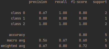
Classification Report
Show the above results in the form of report
code:
from sklearn.metrics import classification_report
y_true = [0, 1, 2, 2, 0]
y_pred = [0, 0, 2, 2, 0]
target_names = ['class 0', 'class 1', 'class 2']
print(classification_report(y_true, y_pred, target_names=target_names))
result:
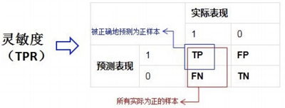
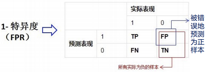
True rate, false positive rate
True rate (TPR) = sensitivity / recall= TP/(TP+FN)TP/(TP+FN) How many samples are detected in the positive example
False positive rate (FPR) = 1-specificity= FP/(FP+TN)FP/(FP+TN) How many samples in the negative example are covered by errors
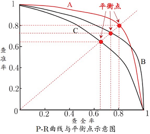
P-R curve
- If the PR curve of one learning algorithm is completely "wrapped" by the curve of another learning algorithm, it can be considered that the performance of the latter is better than the former, such as A is better than C;
- If the PR curves of the two learning algorithms intersect (such as A and B), it is difficult to judge which is better or worse, and can only be compared under the specific conditions of precision and recall;
- By comparing the area under the P-R curve (PR-AUC)
- Use the equilibrium point (i.e. the value when P=R)
- Measure with F1
ROC
AUC
Cost sensitive error rate
slightly