Tip: after the article is written, the directory can be generated automatically. Please refer to the help document on the right for how to generate it
preface
This paper mainly records some classical convolution network architectures and the corresponding pytorch code.
Tip: the following is the main content of this article.
1, LeNet
1.1 network structure and highlights
Network structure:
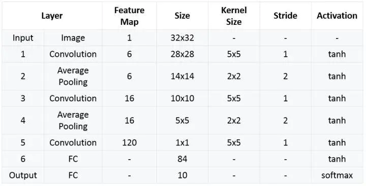
Highlights:
1) Convolutional neural networks use three layers as a series: convolution, pooling, and nonlinearity
2) Extracting spatial features using convolution
3) Use subsample mapped to spatial mean
4) Nonlinearity in hyperbolic (tanh) or S-type (sigmoid) form
6) The sparse connection matrix between layers avoids large computational cost
1.2 code
import torch
import torch.nn.functional as F
import torch.nn as nn
import torch.optim as optim
import torchvision
import matplotlib.pyplot as plt
import numpy as np
from PIL import Image ##Use this library to open pictures and import corresponding data
## display picture
def imshow(img):
    npimg=img.numpy()
    plt.imshow(np.transpose(npimg,(1,2,0))) ## Convert dimensions of pictures
    plt.show()
class LeNet(nn.Module):
    def __init__(self):
        super(LeNet,self).__init__()
        self.conv1=torch.nn.Conv2d(3,16,(5,5))
        self.pool1=torch.nn.MaxPool2d(2,2)  ## If the step size is not specified, it defaults to kersize
        self.conv2=torch.nn.Conv2d(16,32,(5,5))
        self.pool2=torch.nn.MaxPool2d(2,2)
        self.fc1=torch.nn.Linear(32*5*5,120)
        self.fc2=torch.nn.Linear(120,84)
        self.fc3=torch.nn.Linear(84,10)
    def forward(self,X):
        X=F.relu(self.conv1(X))
        X=self.pool1(X)
        X=F.relu(self.conv2(X))
        X=self.pool2(X)
        X=X.view(-1,32*5*5)
        X=F.relu(self.fc1(X))
        X=F.relu(self.fc2(X))
        Z=self.fc3(X)
        return Z
x_test=0
net=LeNet()
loss_func=torch.nn.CrossEntropyLoss()
optimizer=torch.optim.Adam(net.parameters(),lr=0.01)
outputs=0
for epoch in range(500):
    running_loss=0.0
    optimizer.zero_grad() ## If you don't leave it blank, you can calculate the gradient of large batchsize
    if(epoch % 500 ==499):
        with torch.no_grad():  ## Error gradients are not calculated
            outputs=net(x_test)
            predict_y=torch.max(outputs,dim=1)[1] ## Returns the index with the highest probability
            pass
save_path=""
torch.save(net.state_dict(),save_path)  ## Save network parameters
net=LeNet()
net.load_state_dict(torch.load(""))
2, Alex net
2.1 network structure and highlights
Network structure:
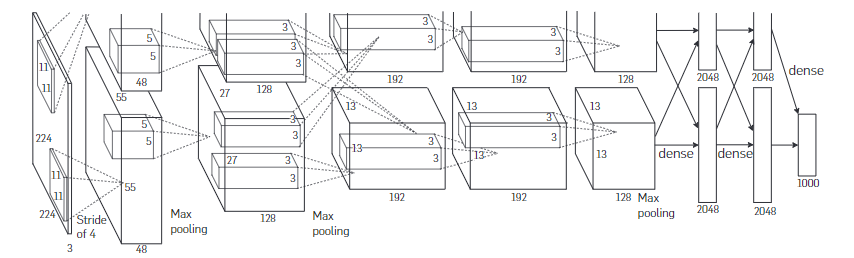
Highlights:
1. All nonlinear activation functions Relu are used
2. The overall architecture of LRN (local normalization layer, which is proved to be ineffective later) overlapping pool network (the convolution kernel of the pool is stripe < kernei_size, which will cause overlapping pooling, which is conducive to preventing over fitting)
3. Prevent over fitting technology, data enhancement and dropout (increase the amount of data and prevent over fitting by randomly intercepting 224 regions from the original image of 256256.)
2.2 code
import torch
import torch.nn as nn
from torch.utils.data import DataLoader
import torch.nn.functional as F
import torchvision.transforms as transforms
import torchvision.datasets as datasets
from tqdm import tqdm
class AlexNet(nn.Module):
    def __init__(self,num_classes=5):
        super(AlexNet,self).__init__()
        self.features=nn.Sequential(
            nn.Conv2d(3,48,kernel_size=11,stride=4,padding=2),
            nn.ReLU(inplace=True),
            nn.MaxPool2d(kernel_size=3,stride=2),
            nn.Conv2d(48,128,kernel_size=5,padding=2),
            nn.ReLU(inplace=True),
            nn.MaxPool2d(kernel_size=3,stride=2),
            nn.Conv2d(128,192,kernel_size=3,padding=1),
            nn.ReLU(inplace=True),
            nn.Conv2d(192,192,kernel_size=3,padding=1),
            nn.ReLU(inplace=True),
            nn.Conv2d(192,128,kernel_size=3,padding=1),
            nn.ReLU(inplace=True),
            nn.MaxPool2d(kernel_size=3,stride=2)
        )
        self.classifier=nn.Sequential(
            nn.Dropout(p=0.5),
            nn.Linear(128*6*6,4096),
            nn.ReLU(inplace=True),
            nn.Dropout(p=0.5),
            nn.Linear(4096,4096),
            nn.ReLU(inplace=True),
            nn.Linear(4096,num_classes)
        )

    def forward(self,x):
        x=self.features(x)
        x=torch.flatten(x,start_dim=1)
        x=self.classifier(x)
        return x
device=torch.device("cuda:0" if torch.cuda.is_available() else "cpu")
data_transform={
    "train":transforms.Compose([transforms.RandomResizedCrop(224),
                                transforms.RandomHorizontalFlip(),
                                transforms.ToTensor(),
                                transforms.Normalize((0.5,0.5,0.5),(0.5,0.5,0.5))
                                ]),
    "val":transforms.Compose([transforms.Resize((224,224)),
                              transforms.ToTensor(),
                              transforms.Normalize((0.5, 0.5, 0.5), (0.5, 0.5, 0.5))
                              ])}

image_path=r'E:/MyCode/pythonProject1/MyPytorch/data_set/flower_data/'
train_data=datasets.ImageFolder(root=image_path+"train",transform=data_transform['train'])
validate_dataset = datasets.ImageFolder(root=image_path+"val",
                                            transform=data_transform["val"])
val_num = len(validate_dataset)
validate_loader = torch.utils.data.DataLoader(validate_dataset,
                                                  batch_size=4, shuffle=False,
                                                  num_workers=0)
flower_index=train_data.class_to_idx
cla_dict=dict((val,key) for key,val in flower_index.items())
batch_size=32
data_loader=DataLoader(train_data,batch_size=batch_size,shuffle=True,num_workers=0)
net=AlexNet()
net.to(device)
loss_func=nn.CrossEntropyLoss()
optimizer=torch.optim.Adam(net.parameters(),lr=0.0002)
best_acc=0.0
epochs = 10
print(device)
for epoch in range(epochs):
    net.train()
    runnning_loss=0.0
    train_steps = len(data_loader)
    train_bar = tqdm(data_loader)
    for step,data in enumerate(train_bar,start=0):
        images,labels=data
        optimizer.zero_grad()
        output=net(images.to(device))
        loss=loss_func(output,labels.to(device))
        loss.backward()
        optimizer.step()
        runnning_loss+=loss.item()
        train_bar.desc = "train epoch[{}/{}] loss:{:.3f}".format(epoch + 1,
                                                                 epochs,
                                                                 loss)
    net.eval()
    acc = 0.0  # accumulate accurate number / epoch
    with torch.no_grad():
        val_bar = tqdm(validate_loader)
        for val_data in val_bar:
            val_images, val_labels = val_data
            outputs = net(val_images.to(device))
            predict_y = torch.max(outputs, dim=1)[1]
            acc += torch.eq(predict_y, val_labels.to(device)).sum().item()
    val_accurate = acc / val_num
    print('[epoch %d] train_loss: %.3f  val_accuracy: %.3f' %
          (epoch + 1, runnning_loss / train_steps, val_accurate))
    if val_accurate > best_acc:
        best_acc = val_accurate
3, VGG
3.1 network structure and highlights
Structure of VGG network
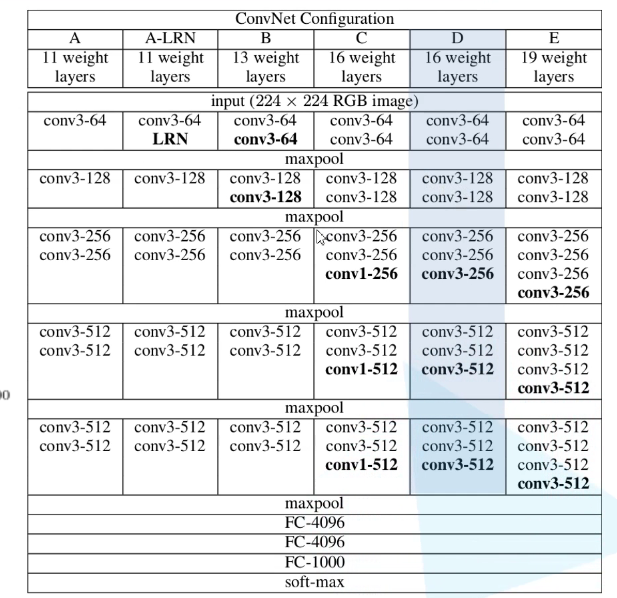
Generally speaking, we use the structure of D. Where, the stripe of conv layer = 1, padding=1
maxpool size=2, stripe = 2
Relevant highlights
1. By stacking multiple 3 * 3 convolution kernels to replace the large-scale convolution kernels (reducing the required parameters), it also has more nonlinear transformations, which increases CNN's ability to learn features. (the alternative structure of multiple convolution layers and nonlinear activation layers can extract deeper and better features than the structure of single convolution layer.)
For example, the convolution kernel of 55 can be replaced by stacking two convolution kernels of 33.
The convolution kernel of 77 can be replaced by stacking three convolution kernels of 33.
The above alternatives have the same receptive field.
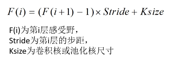
Supplement: CNN receptive field determines the area size of the input layer corresponding to an element in the output result of a layer, which is called receptive field. Generally speaking, a cell on the output feature map corresponds to the area size on the input layer.
The calculation formula of receptive field is as follows:
2. In the convolution structure of VGGNet, 1 * 1 convolution kernel is introduced. Without affecting the input and output dimensions, nonlinear transformation is introduced to increase the expression ability of the network and reduce the amount of calculation.
3. During training, first train the A-level network of VGGNet with simple level (shallow layers), and then use the weight of a-network to initialize the later complex model to speed up the convergence speed of training.
4. Multi scale method is used to train and predict. It can increase the amount of training data, prevent over fitting of the model and improve the prediction accuracy.
Supplement: Multi Size training
Each image is individually scaled by randomly selecting S from [Smin,Smax] (Smin=256, Smax=512). Because the objects in the image may be of various sizes, it is advantageous to adopt this method in training. The first mock exam is also a scale jittering training set data enhancement, which enables a single model to recognize objects of various sizes. Considering the training speed, we use the same configuration of the fixed S=384 pre training model to fine tune all layers of a single-scale model to train the multi-scale model.
5. It is proved that the local normalization layer does not work.
Refer to: overfeat: integrated recognition, localization and detection using revolutionary networks
reference
Very Deep Convolutional Networks for Large-Scale Image Recognition
3.2 code
import torch
import torch.nn.functional as F
import numpy as np
import torch.nn as nn
class VGGNet(nn.Module):
    def __init__(self,features,class_num=1000):
        super(VGGNet,self).__init__()
        self.features=features
        self.classifier=nn.Sequential(
            nn.Dropout(p=0.5),
            nn.Linear(512*7*7,4096),
            nn.ReLU(True),
            nn.Dropout(p=0.5),
            nn.Linear(2048,4096),
            nn.ReLU(True),
            nn.Linear(4096,class_num)
        )
    ## Forward propagation
    def forward(self,x):
        x=self.features(x)
        x=torch.flatten(x,start_dim=1)
        x=self.classifier(x)
        return x
    ## Initialization parameters
    def _initialize_weights(self):
        for m in self.modules():
            if isinstance(m,nn.Conv2d):
                nn.init.xavier_uniform(m.weight)
                if m.bias is not None:
                    nn.init.constant_(m.bias,0)
            if isinstance(m,nn.Linear):
                nn.init.xavier_uniform(m.weight)
                nn.init.constant_(m.bias,0)
## Generating and extracting feature network structure
def make_feature(cfg:list):
    layers=[]
    ## Default input channel
    in_channels=3
    for v in cfg:
        if v=='M':
            layers+=[nn.MaxPool2d(kernel_size=2,stride=(2,2))]
        else:
            conv2d=nn.Conv2d(in_channels,v,kernel_size=(3,3),padding=(1,1))
            layers+=[conv2d,nn.ReLU(True)]
            in_channels=v
    ## Non keyword parameter passed in parameter
    return nn.Sequential(*layers)
## VGGNet configuration parameter dictionary
cfgs={
    'VGG-11':[64,'M',128,'M',256,256,'M',512,512,'M',512,512,'M'],
    'VGG-13':[64,64,'M',128,128,'M',256,256,'M',512,512,'M',512,512,'M'],
    'VGG-16':[64,64,'M',128,128,'M',256,256,256,'M',512,512,512,'M',512,512,512,'M'],
    'VGG-19':[64,64,'M',128,128,'M',256,256,256,256,'M',512,512,512,512,'M',512,512,512,512,'M']
}
def vgg(model_name='vgg-16',**kwargs):
    try:
        cfg=cfgs[model_name]
    except:
        raise BaseException
    ## kwargs variable length dictionary variable
    model=VGGNet(make_feature(cfg),**kwargs)
    return model

## Using gpu training
device=torch.device("cuda:0" if torch.cuda.is_available() else "cpu")
4, GoogLeNet
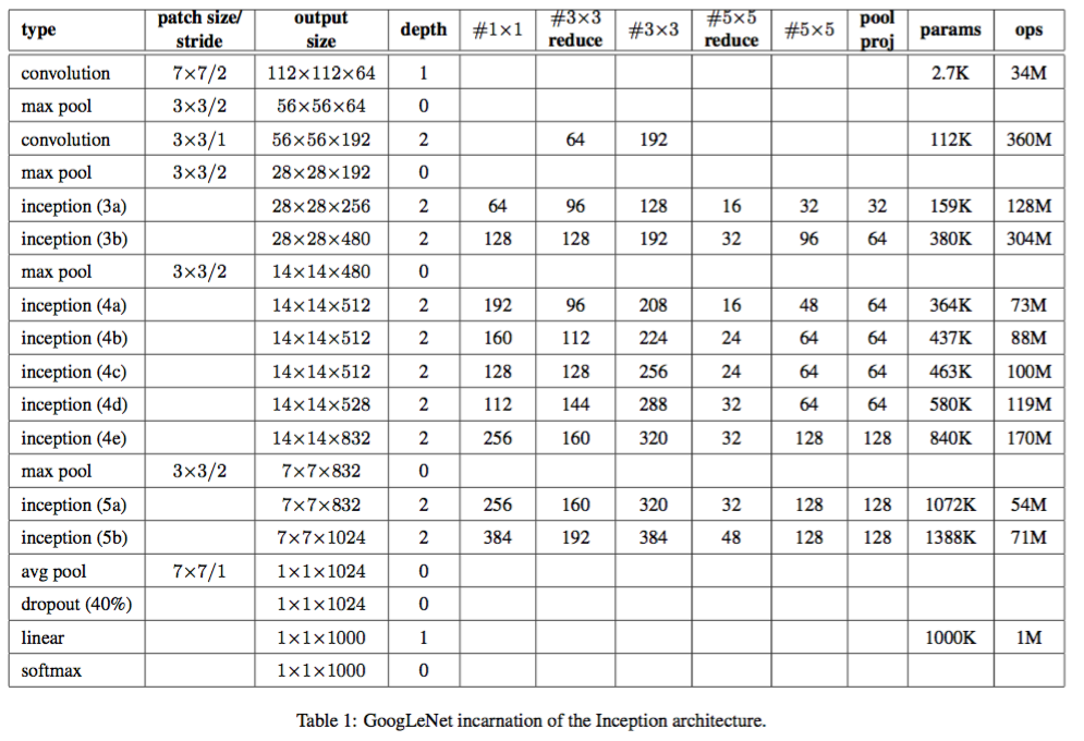
4.1 network structure and highlights
Specific framework of network
Motivation or idea of the paper:
The method of directly improving the depth of neural network is to increase the size of the network, including width and depth. Depth is the number of layers in the network, and width refers to the number of neurons used in each layer. However, this simple and direct solution has two major disadvantages.
(1) The increase of network size also means the increase of parameters, which makes the network easier to over fit.
(2) Increase in computing resources.
This paper solves these two problems by thinking of changing the way of full connection to sparse connection.
When the probability distribution of the data set is expressed by a large and sparse deep neural network, the network topology can be optimized by layer by layer analysis of the activation value of the upper layer highly related to the output and the relevant statistical information of clustering neurons. (Provable bounds for learning some deep representations)
Generally, full connection is to better optimize parallel computing, while sparse connection is to break symmetry to improve learning. Therefore, we consider whether there is a method that can not only maintain the sparsity of network structure, but also make use of the high computing performance of dense matrix. According to the existing literature, clustering sparse matrices into dense sub matrices can improve the computational performance, so the concept structure is proposed.
Relevant highlights:
1. The inception structure is added to increase the width and depth of the network without increasing the computing load.
Add some ideas about inception structure
(1) 1 * 1 convolution kernel:
If more convolutions are superimposed in the receptive field of the same size, more abundant features can be extracted. (Network in Network)
At the same time, the dimension is reduced to reduce the computational complexity.
(2) Reasons for splicing in feature dimension (fusion of feature information of different scales)
The principle of decomposing sparse matrix into dense matrix is used to speed up the convergence speed
Convolution on multiple scales at the same time can extract features of different scales. Richer features also mean that the final classification judgment is more accurate.
2. Two auxiliary classifiers are added to help training
3. Discard the full connection layer and use the average pooling layer (greatly reducing the parameters of the model)
reference
Going Deeper with Convolutions
4.2 code
import telnetlib
import torch
import torchvision.transforms as transforms
import torch.nn.functional as F
import torch.nn as nn
import torchvision.datasets as datasets
from torch.utils.data import DataLoader
from tqdm import tqdm
## Define GooLeNet classes
class GooLeNet(nn.Module):
    def __init__(self,num_classes=1000,use_aux=True):
        super(GooLeNet, self).__init__()
        self.use_aux=use_aux
        self.conv1=BasicConv2d(3,64,kernel_size=7,stride=2,padding=3)
        ## ceil_mode if it is calculated as a decimal, it will be rounded up, and false will be rounded down
        self.maxPool1=nn.MaxPool2d(3,stride=2,ceil_mode=True)
        self.conv2=BasicConv2d(64,64,kernel_size=1)
        self.conv3=BasicConv2d(64,192,kernel_size=3,padding=1)
        self.maxPool2=nn.MaxPool2d(3,stride=2,ceil_mode=True)
        self.inception3a=Inception(192,64,96,128,16,32,32)
        self.inception3b=Inception(256,128,128,192,32,96,64)
        self.maxPool3=nn.MaxPool2d(3,stride=2,ceil_mode=True)
        self.inception4a=Inception(480,192,96,208,16,48,64)
        self.inception4b=Inception(512,160,112,224,24,64,64)
        self.inception4c=Inception(512,128,128,256,24,64,64)
        self.inception4d=Inception(512,112,144,288,32,64,64)
        self.inception4e=Inception(528,256,160,320,32,128,128)
        self.maxPool4=nn.MaxPool2d(kernel_size=3,stride=2,ceil_mode=True)
        self.inception5a=Inception(832,256,160,320,32,128,128)
        self.inception5b=Inception(832,384,192,384,48,128,128)
        if use_aux:
            self.aux1=AuxiliaryClassifier(512,num_classes)
            self.aux2=AuxiliaryClassifier(528,num_classes)
        ## Adaptive height and width of given output matrix
        self.avgPool=nn.AdaptiveAvgPool2d((1,1))
        self.dropout=nn.Dropout(0.4)
        self.fc=nn.Linear(1024,num_classes)
    def forward(self,x):
        x=self.conv1(x)
        x=self.maxPool1(x)
        x=self.conv2(x)
        x=self.conv3(x)
        x = self.maxPool2(x)
        x=self.inception3a(x)
        x=self.inception3b(x)
        x=self.maxPool3(x)
        x=self.inception4a(x)
        if self.training and self.use_aux:
            aux1=self.aux1(x)
        x=self.inception4b(x)
        x=self.inception4c(x)
        x=self.inception4d(x)
        if self.training and self.use_aux:
            aux2=self.aux2(x)
        x=self.inception4e(x)
        x=self.maxPool4(x)
        x=self.inception5a(x)
        x=self.inception5b(x)
        x=self.avgPool(x)
        x=torch.flatten(x,1)
        x=self.dropout(x)
        x=self.fc(x)
        if self.training and self.use_aux:
            return x,aux2,aux1
        return x
## Define auxiliary classifiers
class AuxiliaryClassifier(nn.Module):
    def __init__(self,in_channel,num_classes):
        super(AuxiliaryClassifier,self).__init__()
        self.avgPool=nn.AvgPool2d(kernel_size=5,stride=3)
        self.conv=BasicConv2d(in_channel,128,kernel_size=1)
        self.fc1=nn.Linear(2048,1024)
        self.fc2=nn.Linear(1024,num_classes)
    def forward(self,x):
        x=self.avgPool(x)
        x=self.conv(x)
        x=torch.flatten(x,start_dim=1)
        ## self.training can be modified by model.train() or model.eval()
        x=F.dropout(x,p=0.7,training=self.training)
        x=F.relu(self.fc1(x),inplace=True)
        x=F.dropout(x,p=0.7,training=self.training)
        x=self.fc2(x)
        return x
## Define Inception structure
## ch1v1 is the number of corresponding convolution kernels
class Inception(nn.Module):
    def __init__(self,in_channels,ch1v1,ch3v3red,ch3v3,ch5v5red,ch5v5,pool_proj):
        super(Inception,self).__init__()
        self.branch1=BasicConv2d(in_channels,ch1v1,kernel_size=1)
        self.branch2=nn.Sequential(
            BasicConv2d(in_channels,ch3v3red,kernel_size=1),
            BasicConv2d(ch3v3red,ch3v3,kernel_size=3,padding=1)
        )
        self.branch3=nn.Sequential(
            BasicConv2d(in_channels,ch5v5red,kernel_size=1),
            BasicConv2d(ch5v5red,ch5v5,kernel_size=5,padding=2)
        )
        self.branch4=nn.Sequential(
            nn.MaxPool2d(kernel_size=3,stride=1,padding=1),
            BasicConv2d(in_channels,pool_proj,kernel_size=1)
        )
    def forward(self,x):
        branch1=self.branch1(x)
        branch2=self.branch2(x)
        branch3=self.branch3(x)
        branch4=self.branch4(x)
        outputs=[branch1,branch2,branch3,branch4]
        ## The input parameter is matrix, and the merged dimension here is channel
        return torch.cat(outputs,1)
## Define the basic convolution layer (including activation function)
class BasicConv2d(nn.Module):
    def __init__(self,in_channels,out_channels,**kwargs):
        super(BasicConv2d,self).__init__()
        self.conv=nn.Conv2d(in_channels,out_channels,**kwargs)
        ## inplace increases the amount of computation to reduce memory usage
        self.relu=nn.ReLU(inplace=True)
    def forward(self,x):
        x=self.conv(x)
        x=self.relu(x)
        return x
device = torch.device("cuda:0" if torch.cuda.is_available() else "cpu")
data_transform = {
    "train": transforms.Compose([transforms.RandomResizedCrop(224),
                                 transforms.ToTensor(),
                                 transforms.RandomHorizontalFlip(),
                                 transforms.Normalize((0.5, 0.5, 0.5), (0.5, 0.5, 0.5))]),
    "eval": transforms.Compose([transforms.RandomSizedCrop((224, 224)),
                                transforms.ToTensor(),
                                transforms.Normalize((0.5, 0.5, 0.5), (0.5, 0.5, 0.5))])
}
image_path = r'E:/MyCode/pythonProject1/MyPytorch/data_set/flower_data/'
train_data = datasets.ImageFolder(root=image_path + "train", transform=data_transform['train'])
eval_data = datasets.ImageFolder(root=image_path + "val", transform=data_transform['eval'])
train_num = len(train_data)
eval_num = len(eval_data)
batch_size = 32
train_loader = DataLoader(train_data, batch_size=batch_size, shuffle=True, num_workers=0)
validate_loader = torch.utils.data.DataLoader(eval_data,
                                                  batch_size=batch_size, shuffle=False,
                                                  num_workers=0)
##
net = GooLeNet(num_classes=5)
epoches = 10
loss_func = nn.CrossEntropyLoss()
net.to(device)
optimizer = torch.optim.Adam(net.parameters(), lr=0.0002)
train_steps = len(train_loader)
for epoch in range(epoches):
    net.train()
    running_loss = 0.0
    train_bar = tqdm(train_loader)
    for step, data in enumerate(train_bar,start=0):
        optimizer.zero_grad()
        images,labels=data
        output,aux1,aux2=net(images.to(device))
        loss1=loss_func(output,labels.to(device))
        loss2=loss_func(aux1,labels.to(device))
        loss3=loss_func(aux2,labels.to(device))
        loss = loss1 + loss2 * 0.3 + loss3 * 0.3
        loss.backward()
        optimizer.step()
        running_loss += loss.item()
        train_bar.desc = "train epoch[{}/{}] loss:{:.3f}".format(epoch + 1,
                                                                 epoches,
                                                                 loss)
    net.eval()
    acc = 0.0
    with torch.no_grad():
        val_bar = tqdm(validate_loader)
        for data in val_bar:
            val_images, val_labels = data
            output = net(val_images.to(device))
            predict_y = torch.max(output, dim=1)[1]
            acc += torch.eq(predict_y, val_labels.to(device)).sum().item()
    val_accurate = acc / eval_num
    print('[epoch %d] train_loss: %.3f  val_accuracy: %.3f' %
          (epoch + 1, running_loss / train_steps, val_accurate))
5, ResNet
5.1 network structure and highlights
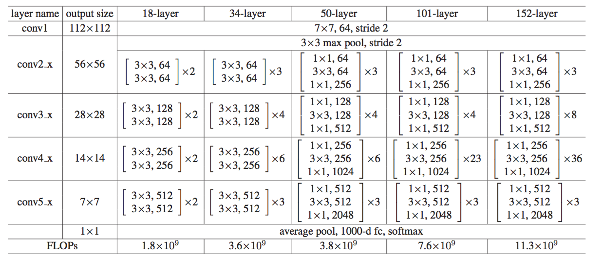
Network structure of ResNet:
Some ideas of the paper
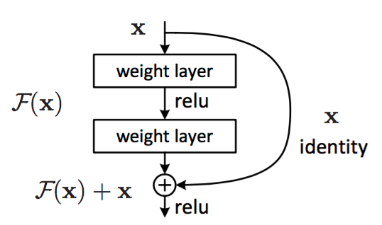
1. When the neural network is deeper, there will be gradient explosion / disappearance. The reason for this is not the over fitting of neural network, but that adding more layers to the appropriate depth model will lead to higher training errors.
In this paper, residual blocks and jump links are used to solve the above problems. That is, residual layers are proposed to explicitly let these layers fit the residual mapping, rather than hoping that every few stacked layers directly fit the desired basic mapping.
Jump connection does not add additional parameters or computational complexity.
Supplement: residual represents:
In image recognition, VLAD is a representation encoded by the residual vector of the dictionary, and Fisher vector can be expressed as the probability version of VLAD. They are powerful shallow representations in image retrieval and image classification. For vector quantization, the coding residual vector is proved to be more effective than the coding original vector.
Jump link: the early practice of training multi-layer perceptron (MLP) was to add a linear layer to connect the input and output of the network.
The residual structure is easier to learn:
1. If the identity mapping is optimal, the solver may simply push the weights of multiple nonlinear connections to zero to approach the identity mapping.
2. In practice, identity mapping is unlikely to be optimal, but our reconstruction may help to preprocess the problem.
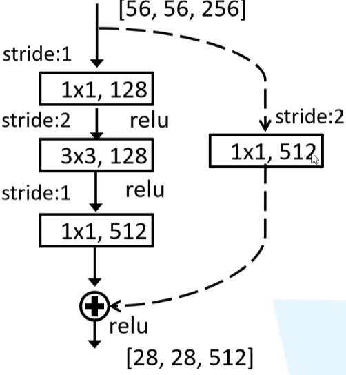
Supplement: Rules for designing network:
1. For layers with the same output feature map size, there are the same number of filters, that is, the number of channel s is the same;
2. When the feature map size is halved (pooled), the number of filters is doubled.
For the residual network, the shortcut connection of dimension matching is a solid line, otherwise it is a dotted line. When dimensions do not match, there are two options for equivalent mapping:
1) Directly increase the dimension (channel) through zero padding.
2) Multiply the W matrix and project it to the new space. The implementation is realized by 1x1 convolution, which directly changes the number of filters of 1x1 convolution. This will increase the parameters.
Highlights
1. Compared with traditional convolutional neural networks such as VGG, the complexity is reduced and the required parameters are reduced.
2. It can be deeper without gradient dispersion.
3. Simple optimization and deeper classification accuracy due to the use of deeper networks.
4. Solve the problem of deep-seated network degradation.
reference:
Deep Residual Learning for Image Recognition
5.2 code
import torch
import torchvision
import torch.nn.functional as F
import torch.nn as nn
from torch.utils.data import DataLoader
import torch.optim as optim
class ResNet(nn.Module):
    ## List of blocks used by block and the number of residual blocks of each conv
    def __init__(self,block,block_num,num_classes=1000):
        super(ResNet,self).__init__()
        ## According to the paper, the default is 64
        self.in_channels=64
        self.conv1=nn.Conv2d(3,self.in_channels,kernel_size=7,stride=2,padding=3,bias=False)
        self.bn1=nn.BatchNorm2d(self.in_channels)
        self.relu=nn.ReLU(inplace=True)
        ## It needs to be the original general, rounded down by default
        self.maxpool=nn.MaxPool2d(kernel_size=3,stride=2,padding=1)
        self.layer1=self._make_layer(block,64,block_num[0])
        self.layer2=self._maker_layer(block,128,block_num[1],stride=2)
        self.layer3=self._maker_layer(block,256,block_num[2],stride=2)
        self.layer4=self._maker_layer(block,512,block_num[3],stride=2)
        self.avgpool=nn.AdaptiveAvgPool2d((1,1))
        self.fc=nn.Linear(512*block.expansion,num_classes)
    def _maker_layer(self,block,channel,block_num,stride=1):
        downsample=None
        if stride!=1 or self.in_channels !=channel*block.expansion:
            downsample=nn.Sequential(
                nn.Conv2d(self.in_channels,channel*block.expansion,kernel_size=1,stride=stride,bias=False),
                nn.BatchNorm2d(channel*block.expansion)
            )
        layers=[]
        layers.append(block(self.in_channels,channel,downsample=downsample,stride=stride))
        self.in_channels=channel*block.expansion
        for _ in range(1,block_num):
            layers.append(block(self.in_channels,channel))
        return nn.Sequential(*layers)
    def forward(self,x):
        x=self.conv(x)
        x=self.bn1(x)
        x=self.relu(x)
        x=self.maxpool(x)
        x=self.layer1(x)
        x=self.layer2(x)
        x=self.layer3(x)
        x=self.layer4(x)
        x=self.avgpool(x)
        x=torch.flatten(x,1)
        x=self.fc(x)
        return x
## Basic residual block of 18 and 30 layers
class BasicBlock(nn.Module):
    ## Whether the number of convolution kernels of residual structure changes. If it is 1, it remains unchanged
    expansion=1
    ## Is there a corresponding dimension modification operation for the sampling shortcut under downsample
    def __init__(self,in_channels,out_channels,stride=1,downsample=None):
        super(BasicBlock,self).__init__()
        self.conv1=nn.Conv2d(in_channels=in_channels,out_channels=out_channels,kernel_size=3,stride=stride,padding=1,bias=False)
        self.bn1=nn.BatchNorm2d(out_channels)
        self.relu=nn.ReLU()
        self.conv2=nn.Conv2d(in_channels=out_channels,out_channels=out_channels,kernel_size=3,stride=1,padding=1,bias=False)
        self.bn2=nn.BatchNorm2d(out_channels)
        self.downsample=downsample
    def forward(self,x):
        identity=x
        if self.downsample is not None:
            identity=self.downsample(x)
        out=self.conv1(x)
        out=self.bn1(out)
        out=self.relu(out)
        out=self.conv2(out)
        out=self.bn2(out)
        out+=identity
        out=self.relu(out)
        return out
## Basic heading of level 50
class Bottleneck(nn.Module):
    ## Similarly, it can be seen from the paper that the number of convolution kernels of the last residual structure of layers 50, 101 and 152 is 4 times that of the previous one, so it is 4
    expansion=4
    def __init__(self,in_channels,out_channels,stride=1,downsample=None):
        super(Bottleneck,self).__init__()
        self.conv1=nn.Conv2d(in_channels=in_channels,out_channels=out_channels,kernel_size=1,stride=1,bias=False)
        self.bn1=nn.BatchNorm2d(out_channels)
        self.conv2=nn.Conv2d(in_channels=out_channels,out_channels=out_channels,kernel_size=3,stride=stride,padding=1,bias=False)
        self.bn2=nn.BatchNorm2d(out_channels)
        self.conv3=nn.Conv2d(in_channels=out_channels,out_channels=out_channels*self.expansion,kernel_size=1,stride=1,bias=False)
        self.bn3=nn.BatchNorm2d(out_channels*self.expansion)
        self.relu=nn.ReLU(inplace=True)
        self.downsample=downsample
    def forward(self,x):
        identity=x
        if self.downsample is not None:
            identity=self.downsample(x)
        out=self.conv1(x)
        out=self.bn1(out)
        out=self.relu(out)
        out=self.conv2(out)
        out=self.bn2(out)
        out=self.relu(out)
        out=self.conv3(out)
        out=self.bn3(out)
        out+=identity
        out=self.downsample(out)
        return out
def resnet34(num_classes=1000):
    return ResNet(BasicBlock,[3,4,6,4],num_classes=num_classes)

def resnet101(num_classes=1000):
    return ResNet(Bottleneck,[3,4,23,3],num_classes=num_classes)
6, MobileNet
6.1 network structure and highlights
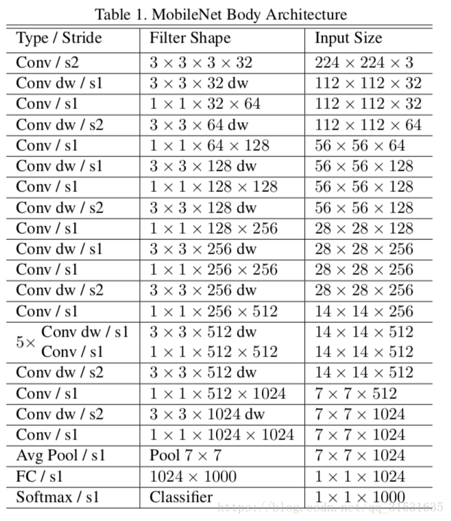
MobileNet_v1 network structure:
Some ideas and motives of the paper:
In order to realize the corresponding computer vision on mobile devices, it is necessary to greatly reduce the parameters required for calculation without greatly reducing the accuracy.
Therefore, a depth separable convolution is proposed, and two model shrinkage super parameters are added at the same time, namely width multiplier and resolution multiplier.
Highlights:
1. Depth separable conv:
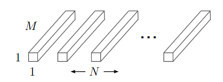
Depth convolution (DW) uses a convolution kernel for each channel, that is, the m-th convolution kernel is applied to the m-th channel in F to generate the convolution output characteristic diagram of the m-th channel. Thus, the amount of parameters required can be greatly reduced.
However, depth convolution only convolutes the input channels, and does not combine them to produce new features. Therefore, it is necessary to add a convolution of 11 to the next layer to calculate a linear combination of the output of the depth convolution, so as to generate new features. (Pointwise Conv,PW)
The depth separable convolution generated by the combination of depth convolution and point-by-point convolution of 1x1 convolution can theoretically reduce the amount of calculation by 8-9 times compared with the standard convolution, and has only a minimal decrease in accuracy.
2. The hyperparametric width multiplier is added α, Resolution multiplier β.
Where width multiplier α: It is mainly to thin each layer so that the number of input channels and output channels are the same α Times, generally set to 1 \ 0.75 \ 0.5 \ 0.25. (experiments show that thinning operation is better than shallow operation)
Resolution multiplier β: Set the resolution size of the input, i.e β DF.
MobileNet_v2:
Some ideas and motives of the paper:
Optimize MobileNet_v1, I hope it can have better accuracy under the condition of smaller amount of data.
Network structure:
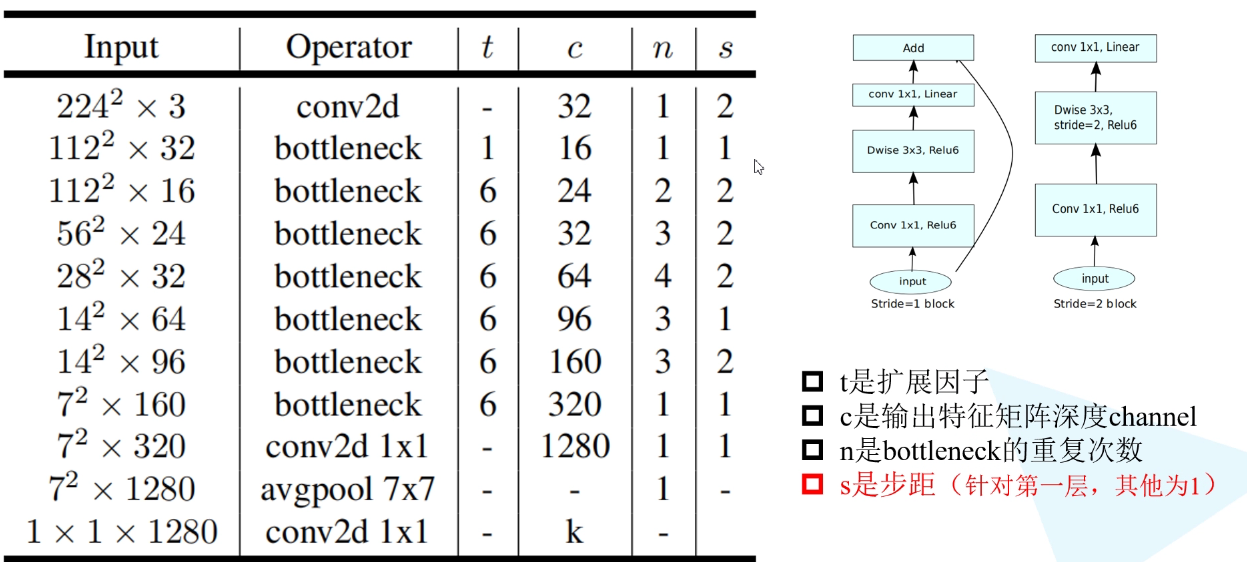
Highlights:
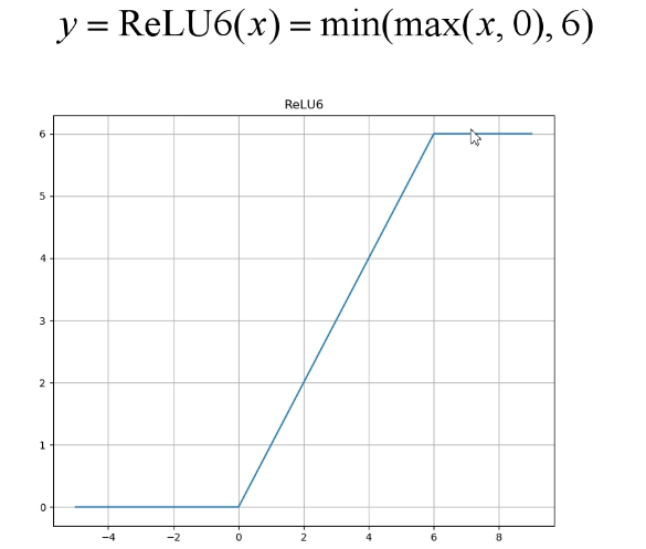
1. inverted residual structure: first expand the input from low dimension to high dimension, then filter it with depth convolution, and then compress it from high dimension to low dimension. At the same time, relu6 activation function is used.
2.Linear Bottlenecks
We believe that in neural networks, the corresponding manifest of interest (translated as popular interest, i.e. formed through a series of convolution and activation layers) can be embedded into low-dimensional subspaces.
Supplement: in a sense, the width control factor of MobileNetv1 α It also controls the dimension of the active space so that the manifest of interest spans the entire space.
However, if the manifest of interest in the current activation space has high integrity, some information will be lost through Relu.
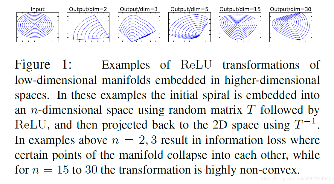
From the above figure, we can see that for low latitude, Relu will lose a lot of information.
Therefore, we know that if we want to keep the manifest of interest completely in the low dimensional space, relu is likely to filter out a lot of useful information, and for the parts that are not filtered, relu is a linear classifier.
Therefore, linear bottleneck is proposed to replace Relu's nonlinear activation transform.
Supplement: if the manifest of interest can be embedded into a significant low dimensional subspace through the activation space, usually the ReLU transform can retain information
reference
1.MobileNets: Efficient Convolutional Neural Networks for MobileVision Applications
2.MobileNetV2: Inverted Residuals and Linear Bottlenecks
6.2 code
import torch
import torch.nn as nn
import torch.nn.functional as F
import numpy as np
import torch.optim as optim
class ConvBNReLu(nn.Sequential):
    def __init__(self,in_channels,out_channels,kernel_size=3,stride=1,groups=1):
        padding=(kernel_size-1)//2
        super(ConvBNReLu,self).__init__(nn.Conv2d(in_channels=in_channels,out_channels=out_channels,kernel_size=kernel_size,stride=stride,groups=groups,bias=False,padding=padding),
                                        nn.BatchNorm2d(out_channels),
                                        nn.ReLU6(inplace=True)
                                        )

class InvertResidual(nn.Module):
    ## expand_ratio expansion factor
    def __init__(self,in_channel,out_channel,stride,expand_ratio):
        super(InvertResidual,self).__init__()\
        ## tk
        hidden_channel=in_channel*expand_ratio
        ## Use shortcut
        self.use_shortcut=stride==1 and in_channel==out_channel
        layers=[]
        if expand_ratio!=1:
            ## Add a 1 * 1 dimension increasing convolution
            layers.append(ConvBNReLu(in_channel,hidden_channel,kernel_size=1))
        layers.extend([
            ##dw convolution
            ConvBNReLu(hidden_channel,hidden_channel,kernel_size=3,stride=stride,groups=hidden_channel),
            ## Linear activation function is used
            nn.Conv2d(hidden_channel,out_channel,kernel_size=1,bias=False),
            nn.BatchNorm2d(out_channel)
        ])
        self.conv=nn.Sequential(*layers)
    def forward(self,x):
        if self.use_shortcut:
            return x+self.conv(x)
        else:
            return self.conv(x)
## min_ Minimum number of channel s used by Ch
def _make_divisible(ch,divisor=8,min_ch=None):
    if min_ch is None:
        min_ch=divisor
    ## Adjust the input channels to the nearest integer multiple of 8. When ch=12, it is 16
    new_ch=max(min_ch,int(ch+divisor/2)//divisor*divisor)
    ## The adjusted channel cannot be reduced by more than 10%
    if new_ch<0.9*ch:
        new_ch+=divisor
    return new_ch
class MobileNetV2(nn.Module):
    def __init__(self,num_classes=1000,alpha=1.0,round_nearest=8):
        super(MobileNetV2,self).__init__()
        block=InvertResidual
        ## Adjust the entered dimension to an integer multiple of the dimension roundnestest
        input_channels=_make_divisible(32*alpha,round_nearest)
        last_channels=_make_divisible(1280*alpha,round_nearest)
        ## Parameter setting of residual block
        inverted_residual_setting=[
            [1,16,1,1],
            [6,24,2,2],
            [6,32,3,2],
            [6,64,4,2],
            [6,96,3,1],
            [6,160,3,2],
            [6,320,1,1],
        ]
        features=[]
        features.append(ConvBNReLu(3,input_channels,stride=2))
        for t,c,n,s in inverted_residual_setting:
            ## Adjust the output channel of each layer
            output_channel=_make_divisible(c*alpha,round_nearest)
            for i in range(n):
                ## s is the stripe of the first layer of each residual structure, and the subsequent ones are 1
                stride=s if i==0 else 1
                features.append(block(input_channels,output_channel,stride,expand_ratio=t))
                input_channels=output_channel

        features.append(ConvBNReLu(input_channels,last_channels,1))
        self.features=nn.Sequential(*features)
        self.avgpool=nn.AdaptiveAvgPool2d((1,1))
        ## Full connection layer
        ## Or you can directly use Conv2d according to the paper structure. The effect of Conv2d and linear is the same
        # self.classifier=nn.Sequential(
        #     nn.Conv2d(last_channels,num_classes,kernel_size=1,stride=1)
        # )
        self.classifier=nn.Sequential(
            nn.Dropout(0.2),
            nn.Linear(last_channels,num_classes)
        )
    def forward(self,x):
        x=self.features(x)
        x=self.avgpool(x)
        x=torch.flatten(x,1)
        x=self.classifier(x)
        return x
Supplement: not every residual structure has a shortcut, but only when stripe = 1 and the input characteristic matrix is the same as the output characteristic matrix shape.