Decision tree is a basic classification and regression method. This chapter mainly discusses the decision tree for classification. The decision tree model has a tree structure. In the classification problem, it represents the process of classifying instances based on features. It can be considered as a set of if then rules, or as a conditional probability distribution defined in feature space and class space. Its main advantage is that the model has readability and fast classification speed. When learning, the decision tree model is established by using the training data and the principle of minimizing the loss function. When forecasting, the new data are classified by decision tree model. Decision tree learning usually includes three steps: feature selection, decision tree generation and decision tree pruning.
5.1 decision tree model and learning
5.1.1 decision tree model
Definition (decision tree)
Classification decision tree model is a tree structure that describes the classification of instances. The decision tree consists of nodes and directed edges. There are two types of nodes: internal nodes and leaf nodes. An internal node represents a feature or attribute, and a leaf node represents a class.
Using decision tree classification, start from the root node, test a feature of the instance, and assign the instance to its child nodes according to the test results: at this time, each child node corresponds to a value of the feature. In this way, the instance is tested and allocated recursively until it reaches the leaf node. Finally, the instance is divided into leaf node classes.
5.1.2 decision tree and if then rules
The decision tree can be regarded as a set of if then rules. The process of transforming the decision tree into if then rules is as follows: a rule is constructed from each path from the root node to the leaf node of the decision tree; The characteristics of internal nodes on the path correspond to the conditions of the rule, while the classes of leaf nodes correspond to the conclusions of the rule. The path of decision tree or its corresponding if then rule set has an important property: mutual exclusion and completeness. That is, each instance is covered by a path or a rule, and only by a path or a rule. Here, the so-called coverage means that the characteristics of the instance are consistent with those on the path, or the instance meets the conditions of the rule.
5.1.3 decision tree and conditional probability distribution
The decision tree also represents the conditional probability distribution of a class under a given characteristic condition. This conditional probability distribution is defined on a partition of the feature space. The feature space is divided into disjoint units or regions, and a class probability distribution is defined in each unit to form a conditional probability distribution. A path of the decision tree corresponds to a unit in the partition. The conditional probability distribution represented by the decision tree consists of the conditional probability distribution of the class under the given conditions of each unit.
5.1.4 decision tree learning
Suppose a given training data set
D = { ( x 1 , y 1 ) , ( x 2 , y 2 ) , ... , ( x N , y N ) } D=\{(x_1,y_1),(x_2,y_2),\dots,(x_N,y_N)\} D={(x1,y1),(x2,y2),...,(xN,yN)}
Among them, x i = ( x i ( 1 ) , x i ( 2 ) , ... , x i ( n ) ) T x_i=(x^{(1)}_{i},x^{(2)}_{i},\dots,x^{(n)}_{i})^{T} xi = (xi(1), xi(2),..., xi(n)) T is the input instance (eigenvector), n n n is the number of features, y i ∈ { 1 , 2 , ... , K } y_i \in \{1,2,\dots,K\} yi ∈ {1,2,..., K} is a class tag, N N N is the sample size. The goal of decision tree learning is to build a decision tree model according to the given training data set, so that it can correctly classify instances.
Decision tree learning essentially induces a set of classification rules from the training data set. There may be multiple or none decision trees that do not contradict the training data set (i.e. decision trees that can correctly classify the training data). What we need is a decision tree with less contradiction with the training data and good generalization ability. From another point of view, decision tree learning is to estimate the conditional probability model from the training data set. There are infinite conditional probability models of classes based on feature space division. The conditional probability model we choose should not only fit the training data well, but also predict the unknown data well. Decision tree learning uses loss function to represent this goal.
5.2 feature selection
5.2.1 feature selection
Feature selection is to select the features that have the ability to classify the training data. This can improve the efficiency of decision tree learning. If the result of classification using a feature is not very different from that of random classification, it is said that this feature has no classification ability. Empirically, such characteristics have little effect on the accuracy of decision tree learning. Usually, the criterion of feature selection is information gain or information gain ratio.
5.2.2 information gain
In information theory and probability statistics, entropy is a measure of uncertainty of random variables. set up X X X is a discrete random variable with finite values, and its probability distribution is
P ( X = x i ) = p i , i = 1 , 2 , ... , n P(X=x_i)=p_i,\quad i=1,2,\dots,n P(X=xi)=pi,i=1,2,...,n
Then random variable X X The entropy of X is defined as
H ( X ) = − ∑ i = 1 n p i log p i H(X)=-\sum^{n}_{i=1}p_i\log p_i H(X)=−i=1∑npilogpi
Generally, the logarithm in the above formula is based on 2 or e. at this time, the unit of entropy is called bit or NAT respectively. The greater the entropy, the greater the uncertainty of random variables. Verifiable from definition
0 ≤ H ( p ) ≤ log n 0 \le H(p) \le \log n 0≤H(p)≤logn
random variable X X X random variable under given conditions Y Y Conditional entropy of Y H ( Y ∣ X ) H(Y|X) H(Y ∣ X), defined as X X X under given conditions Y Y Entropy pair of conditional probability distribution of Y X X Mathematical expectation of X
H ( Y ∣ X ) = ∑ i = 1 n p i H ( Y ∣ X = x i ) H(Y|X)=\sum^{n}_{i=1}p_iH(Y|X=x_i) H(Y∣X)=i=1∑npiH(Y∣X=xi)
Information gain representation feature X X The information of X makes the class Y Y The degree to which the uncertainty of Y's information is reduced.
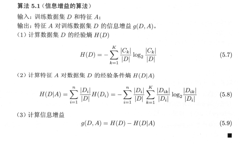
Definition (information gain)
features A A A pair of training data sets D D Information gain of D g ( D , A ) g(D,A) g(D,A), defined as a set D D Empirical entropy of D H ( D ) H(D) H(D) and characteristics A A A under given conditions D D Empirical conditional entropy of D H ( D ∣ A ) H(D|A) Difference of H(D ∣ A), i.e
g ( D , A ) = H ( D ) − H ( D ∣ A ) g(D,A)=H(D)-H(D|A) g(D,A)=H(D)−H(D∣A)
According to the information gain criterion, the feature selection method is to select the training data set D D D. Calculate the information gain of each feature, compare their sizes, and select the feature with the largest information gain.
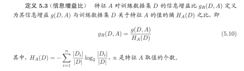
5.2.3 information gain ratio
Taking the information gain as the feature of dividing the training data set, there is a problem of choosing the feature with more values. This problem can be corrected by using the information gain ratio. This is another criterion for feature selection.
5.3 generation of decision tree
5.3.1 ID3 algorithm
The core of ID3 algorithm is to apply the information gain criterion to select features on each node of the decision tree and construct the decision tree recursively.
The specific method is as follows: starting from the root node, calculate the information gain of all possible features for the node, select the feature with the largest information gain as the feature of the node, and establish sub nodes according to the different values of the feature; Then recursively call the above methods to the child nodes to construct the decision tree; Until the information gain of all features is small or no features can be selected. Finally, a decision tree is obtained. ID3 is equivalent to the selection of probability model by maximum likelihood method.
Algorithm (ID3 algorithm)
Input: training dataset D D D. Feature set A A A threshold ε \varepsilon ε;
Output: Decision Tree T T T.
(1) If
D
D
All instances in D belong to the same class
C
k
C_k
Ck, then
T
T
T is a single node tree, and the class
C
k
C_k
Ck , as the node
Class tag, return
T
T
T;
(2) If
A
=
∅
A= \varnothing
A = ∅, then
T
T
T is a single node tree, and
D
D
Class with the largest number of instances in D
C
k
C_k
Ck , as the class of this node
Tag, return
T
T
T;
(3) Otherwise, calculate according to algorithm 5.1
A
A
Each feature pair in A
D
D
D information gain, select the characteristic with the largest information gain
sign
A
g
A_g
Ag;
(4) If
A
g
A_g
The information gain of Ag ^ is less than the wide value
ε
\varepsilon
ε, Then set
T
T
T is a single node tree, and
D
D
Maximum number of instances in D
Class of
C
k
C_k
Ck , as the class mark of the node, returns
T
T
T;
(5) Otherwise, yes
A
g
A_g
Every possible value of Ag +
a
i
a_i
ai, Yi
A
g
=
a
i
A_g =a_i
Ag = ai
D
D
D is divided into several non empty subsets
D
i
D_i
Di, will
D
i
D_i
The class with the largest number of instances in Di , is used as a marker to construct child nodes, which form a tree from nodes and their child nodes
T
T
T. Return
T
T
T;
(6) On the first
i
i
i child node, in
D
i
D_i
Di , is the training set
A
−
{
A
g
}
A-\{A_g\}
A − {Ag} is the feature set, and step (1) is called recursively~
Step (5), get the subtree
T
i
T_i
Ti, return
T
i
T_i
Ti.
ID3 algorithm only generates trees, so the trees generated by this algorithm are prone to over fitting.
from math import log

def createDataSet():
    dataSet = [[1, 1, 'yes'], [1, 1, 'yes'], [1, 0, 'no'], [0, 1, 'no'], [0, 1, 'no']]
    labels = ['no surfacing', 'flippers']
    return dataSet, labels

myDat, myLab = createDataSet()

# Calculating information entropy
def calcShannonEnt(dataSet):
    numEntries = len(dataSet)
    # Create a dictionary for all categories
    labelCounts = {}
    for featVec in dataSet:
        currentLabel = featVec[-1]  # Get the last column of data
        if currentLabel not in labelCounts.keys():
            labelCounts[currentLabel] = 0
        labelCounts[currentLabel] += 1
    # Calculate Shannon entropy
    shannonEnt = 0.0
    for key in labelCounts:
        prob = float(labelCounts[key]) / numEntries
        shannonEnt -= prob * log(prob, 2)
    return shannonEnt

# print(calcShannonEnt(myDat))

# Divide the data set according to the maximum information gain

# Defines a function splitDataSet divided by a feature
# Input three variables (dataset to be divided, feature, classification value)
def splitDataSet(dataSet, axis, value):
    retDataSet = []
    for featVec in dataSet:
        if featVec[axis] == value:
            reduceFeatVec = featVec[:axis]
            reduceFeatVec.extend(featVec[axis + 1:])
            retDataSet.append(reduceFeatVec)
    return retDataSet  # Returns a subset without partition characteristics

# Defines a function that divides data according to the maximum information gain
def chooseBestFeatureToSplit(dataSet):
    numFeature = len(dataSet[0]) - 1
    baseEntropy = calcShannonEnt(dataSet)  # Shannon entropy
    bestInformGain = 0
    bestFeature = -1
    for i in range(numFeature):
        featList = [number[i] for number in dataSet]  # Get all values under a feature (a column)
        uniquelyVales = set(featList)  # set no duplicate attribute eigenvalues
        newEntropy = 0
        for value in uniquelyVales:
            subDataSet = splitDataSet(dataSet, i, value)
            prob = len(subDataSet) / float(len(dataSet))  # p(t)
            newEntropy += prob * calcShannonEnt(subDataSet)  # Sum Shannon entropy of each subset
        infoGain = baseEntropy - newEntropy  # Calculate information gain
        # Maximum information gain
        if infoGain > bestInformGain:
            bestInformGain = infoGain
            bestFeature = i
    return bestFeature  # Return characteristic value
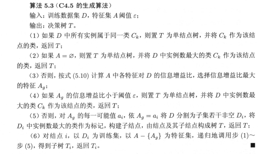
5.3.2 generation algorithm of C4.5
C4.5 algorithm is similar to ID3 algorithm. C4.5 algorithm improves ID3 algorithm. C4.5 in the process of generation, the information gain ratio is used to select features.
5.4 pruning of decision tree
The decision tree generation algorithm recursively generates the decision tree until it cannot continue. The tree generated in this way is often very accurate in the classification of training data, but it is not so accurate in the classification of unknown test data, that is, there is a fitting phenomenon. The reason for over fitting is that too much consideration is given to how to improve the correct classification of training data, so as to construct an overly complex decision tree. The solution to this problem is to consider the complexity of the decision tree and simplify the generated decision tree.
The process of simplifying the generated tree in decision tree learning is called pruning. Specifically, pruning cuts some subtrees or leaf nodes from the generated tree, and takes its root node or parent node as a new leaf node, so as to simplify the classification tree model.
Decision tree pruning is often realized by minimizing the loss function or cost function of the whole decision tree. Set tree T T The number of leaf nodes of T is ∣ T ∣ |T| ∣T∣ , t t t is a tree T T The leaf node of T, which has N t N_t Nt = sample points, where k k The sample points of class k are N t k N_{tk} Ntk , Nos, k = 1 , 2 , ⋯ , K k = 1,2,\cdots ,K k=1,2,⋯,K , H t ( T ) H_t(T) Ht (T) is the leaf node t t Empirical entropy on t, α ≥ 0 \alpha \ge 0 α ≥ 0 is a parameter, then the loss function of decision tree learning can be defined as
C α ( T ) = ∑ t = 1 ∣ T ∣ N t H t ( T ) + α ∣ T ∣ C_\alpha(T)=\sum^{|T|}_{t=1}N_tH_t(T)+\alpha|T| Cα(T)=t=1∑∣T∣NtHt(T)+α∣T∣
H t ( T ) = − ∑ k N t k N t log N t k N t H_{t}(T)=-\sum_{k} \frac{N_{t k}}{N_{t}} \log \frac{N_{t k}}{N_{t}} Ht(T)=−k∑NtNtklogNtNtk
In the loss function, the first term at the right end of the equation is recorded as
C ( T ) = ∑ t = 1 ∣ T ∣ N t H t ( T ) = − ∑ t = 1 ∣ T ∣ ∑ k = 1 K N t k log N t k N t C(T)=\sum_{t=1}^{|T|} N_{t} H_{t}(T)=-\sum_{t=1}^{|T|} \sum_{k=1}^{K} N_{t k} \log \frac{N_{t k}}{N_{t}} C(T)=t=1∑∣T∣NtHt(T)=−t=1∑∣T∣k=1∑KNtklogNtNtk
At this time
C α ( T ) = C ( T ) + α ∣ T ∣ C_\alpha(T)=C(T)+\alpha|T| Cα(T)=C(T)+α∣T∣
C ( T ) C(T) C(T) represents the prediction error of the model on the training data, that is, the fitting degree between the model and the training data, ∣ T ∣ |T| ∣ T ∣ represents model complexity and parameter α ≥ 0 \alpha \ge0 α ≥ 0 to control the influence between the two. Larger α \alpha α Promote the selection of simpler models (trees) and smaller ones α \alpha α Promote the selection of more complex models (trees). α = 0 \alpha=0 α= 0 means that only the fitting degree between the model and the training data is considered, and the complexity of the model is not considered.
Pruning is when α \alpha α When determining, select the model with the smallest loss function, that is, the subtree with the smallest loss function. When α \alpha α When the value is determined, the larger the subtree, the better the fitting with the training data, but the higher the complexity of the model; On the contrary, the smaller the subtree, the lower the complexity of the model, but it often does not fit well with the training data. The loss function just represents the balance between the two.
Algorithm (tree pruning algorithm)
Input: generate the entire tree generated by the algorithm T T T. Parameters α \alpha α;
Output: subtree after construction T α T_\alpha Tα.
(1) Calculate the empirical entropy of each node.
(2) Recursively retract upward from the leaf node of the tree.
If so C α ( T A ) ≤ C α ( T B ) C_\alpha(T_A) \le C_\alpha(T_B) C α (TA)≤C α (TB), prune, that is, change the parent node into a new leaf node
Note that the above formula only needs to consider the difference of the loss function of the two trees, and its calculation can be carried out locally. Therefore, the pruning algorithm of decision tree can be realized by a dynamic programming algorithm.
(3) Return to (2) until the position cannot be continued to obtain the subtree with the smallest loss function T α T_\alpha Tα.
5.5 CART algorithm
Classification and regression tree (CART) model is a widely used decision tree learning method. Cart is also composed of feature selection, tree generation and pruning, which can be used for both classification and regression. The following trees used for classification and regression are collectively referred to as decision trees.
CART is a random variable at a given input X X Output random variable under X condition Y Y Learning method of conditional probability distribution of Y. CART assumes that the decision tree is a binary tree, the values of internal node characteristics are "yes" and "no", the left branch is the branch with the value of "yes", and the right branch is the branch with the value of "no". Such a decision tree is equivalent to recursively bisecting each feature, dividing the input space, that is, the feature space into finite units, and determining the predicted probability distribution on these units, that is, the conditional probability distribution output under the given input conditions.
CART algorithm consists of the following two steps:
(1) Decision tree generation: generate a decision tree based on the training data set, and the generated decision tree should be as large as possible
(2) Decision tree pruning: prune the generated tree with the verification data set and select the optimal subtree. At this time, the minimum loss function is used as the standard of pruning technology.
import operator

def createDataSet1():
    """
    Create sample data/Read data
    @return dataSet labels: Data set collection
    """
    # data set
    originDataSet = [('youth', 'no', 'no', 'commonly', 'disagree'),
                     ('youth', 'no', 'no', 'good', 'disagree'),
                     ('youth', 'yes', 'no', 'good', 'agree'),
                     ('youth', 'yes', 'yes', 'commonly', 'agree'),
                     ('youth', 'no', 'no', 'commonly', 'disagree'),
                     ('middle age', 'no', 'no', 'commonly', 'disagree'),
                     ('middle age', 'no', 'no', 'good', 'disagree'),
                     ('middle age', 'yes', 'yes', 'good', 'agree'),
                     ('middle age', 'no', 'yes', 'very nice', 'agree'),
                     ('middle age', 'no', 'yes', 'very nice', 'agree'),
                     ('old age', 'no', 'yes', 'very nice', 'agree'),
                     ('old age', 'no', 'yes', 'good', 'agree'),
                     ('old age', 'yes', 'no', 'good', 'agree'),
                     ('old age', 'yes', 'no', 'very nice', 'agree'),
                     ('old age', 'no', 'no', 'commonly', 'disagree')]
    # Feature set
    originLabels = ['Age', 'Have a job', 'Have a house', 'Credit situation']
    return originDataSet, originLabels

def calcProbabilityEnt(entDataSet):
    """
    Probability that the sample point belongs to the first class p,I.e. calculation 2 p(1-p)Medium p
    @param entDataSet: data set
    @return probabilityEnt: Probability of data set
    """
    numEntries = len(entDataSet)  # Number of data pieces
    feaCounts = 0
    fea1 = entDataSet[0][len(entDataSet[0]) - 1]
    for featVec in entDataSet:  # Data per row
        if featVec[-1] == fea1:
            feaCounts += 1
    probabilityEnt = float(feaCounts) / numEntries
    return probabilityEnt

def splitDataSet(splitData, index, value):
    """
    Divide the data set and extract all data containing a certain attribute of a certain feature
    @param splitData: data set
    @param index: The characteristic column corresponding to the attribute value
    @param value: A property value
    @return retDataSet: A dataset containing an attribute of a feature
    """
    retDataSet = []
    for featVec in splitData:
        # If the attribute value of the feature of the sample is equal to the incoming attribute value, remove the attribute and put it into the dataset
        if featVec[index] == value:
            reducedFeatVec = featVec[:index] + featVec[index + 1:]  # Remove the current sample of this attribute
            retDataSet.append(reducedFeatVec)  # append appends a new element to the end. The format of the new element in the element remains unchanged. For example, the array exists in the element as a value
    return retDataSet

def chooseBestFeatureToSplit(chooseDataSet):
    """
    Select the optimal feature
    @param chooseDataSet: data set
    @return bestFeature: Optimal feature column
    """
    numFeatures = len(chooseDataSet[0]) - 1  # Total number of features
    if numFeatures == 1:  # When there is only one feature
        return 0
    bestGini = 1  # Optimum Gini coefficient
    bestFeature = -1  # Optimal feature
    for i in range(numFeatures):
        uniqueVales = set(example[i] for example in chooseDataSet)  # De duplication, each attribute value is unique
        feaGini = 0  # Gini coefficient that defines the value of the characteristic
        # The entropy of each eigenvalue is calculated in turn
        for value in uniqueVales:
            subDataSet = splitDataSet(chooseDataSet, i, value)  # Classes classified according to the characteristic attribute value
            # Parameters: original data, cycle times (column of current attribute value), current attribute value
            prob = len(subDataSet) / float(len(chooseDataSet))
            probabilityEnt = calcProbabilityEnt(subDataSet)
            feaGini += prob * (2 * probabilityEnt * (1 - probabilityEnt))
        if feaGini < bestGini:  # The smaller the Gini coefficient, the better
            bestGini = feaGini
            bestFeature = i
    return bestFeature

def majorityCnt(classList):
    """
    For the last feature classification, the category with the most occurrences is the attribute category. For example, if it is finally classified as 2 men and 1 woman, it is determined as male
    @param classList: A dataset is also a category set
    @return sortedClassCount[0][0]: The category of the attribute
    """
    classCount = {}
    # Calculate the number of occurrences of each category
    for vote in classList:
        try:
            classCount[vote] += 1
        except KeyError:
            classCount[vote] = 1
    sortedClassCount = sorted(classCount.items(), key=operator.itemgetter(1), reverse=True)  # The category with the most occurrences is in the first place
    # For the first parameter, sort according to the first field of the parameter (the second parameter), and then reverse the order (the third parameter)
    return sortedClassCount[0][0]  # The category of the attribute

def createTree(treeDataSet, treeLabels):
    """
    For the last feature classification, it is sorted by the number of categories after classification. For example, if the final classification is 2 agree and 1 disagree, it is determined as agree
    @param treeDataSet: data set
    @param treeLabels: Feature set
    @return myTree: Decision tree
    """
    classList = [example[-1] for example in treeDataSet]  # Get the last value of each row of data, that is, the category of each row of data
    # When a dataset has only one category
    if classList.count(classList[0]) == len(classList):
        return classList[0]
    # When the dataset has only one column (i.e. category), it is classified according to the last feature
    if len(treeDataSet[0]) == 1:
        return majorityCnt(classList)
    # Other situations
    bestFeat = chooseBestFeatureToSplit(treeDataSet)  # Select the best feature (in the column)
    bestFeatLabel = treeLabels[bestFeat]  # Optimal feature
    del (treeLabels[bestFeat])  # Deletes the current best feature from the feature set
    uniqueVales = set(example[bestFeat] for example in treeDataSet)  # Select the unique value of the attribute corresponding to the optimal feature
    myTree = {bestFeatLabel: {}}  # The classification results are saved in the form of a dictionary
    for value in uniqueVales:
        subLabels = treeLabels[:]  # For deep copy, the copied value is independent of the original value (ordinary copy is a shallow copy, and changes to the original value or the copied value affect each other)
        myTree[bestFeatLabel][value] = createTree(splitDataSet(treeDataSet, bestFeat, value), subLabels)  # Recursive call to create decision tree
    return myTree

if __name__ == '__main__':
    dataSet, labels = createDataSet1()  # Create presentation data
    print(createTree(dataSet, labels))  # Output decision tree model results