Chapter 6 Logistic Regression and Maximum Entropy Model

Keywords: IIS

Logistic Regression and Maximum Entropy Model

Notes on Li Hang's Statistical Learning Methods Chapter 6 logistic regression and Maximum Entropy Model (2). Maximum Entropy Model

1. Logistic Distribution

Binomial logistic regression model is a classification model, which is expressed by conditional probability distribution P(X Y) P(X Y) P(X Y), in the form of parameterized logistic distribution. Here the random variable takes the real number. Random variable YYY is either 1 or 0.

1.1 LR Bi-Classification Model

P(Y=1∣x)=exp⁡(w⋅x)1+exp⁡(w⋅x)=exp⁡(w⋅x)/exp⁡(w⋅x)(1+exp⁡(w⋅x))/(exp⁡(w⋅x))=1e−(w⋅x)+1P(Y=0∣x)=11+exp⁡(w⋅x)=1−11+e−(w⋅x)=e−(w⋅x)1+e−(w⋅x) \begin{aligned} P(Y=1 | x) &=\frac{\exp (w \cdot x)}{1+\exp (w \cdot x)} \\ &=\frac{\exp (w \cdot x) / \exp (w \cdot x)}{(1+\exp (w \cdot x)) /(\exp (w \cdot x))} \\ &=\frac{1}{e^{-(w \cdot x)}+1} \\ P(Y=0 | x) &=\frac{1}{1+\exp (w \cdot x)} \\ &=1-\frac{1}{1+e^{-(w \cdot x)}} \\ &=\frac{e^{-(w \cdot x)}}{1+e^{-(w \cdot x)}} \end{aligned} P(Y=1∣x)P(Y=0∣x)=1+exp(w⋅x)exp(w⋅x)=(1+exp(w⋅x))/(exp(w⋅x))exp(w⋅x)/exp(w⋅x)=e−(w⋅x)+11=1+exp(w⋅x)1=1−1+e−(w⋅x)1=1+e−(w⋅x)e−(w⋅x)

So the above logistic regression is a linear classification model. The difference between it and linear regression is that in order to reduce the output of linear regression to a large range of numbers, such as from negative infinity to positive infinity, between 0 and 1, such output value can be expressed as "possibility" to convince the general public. Of course, it's also a good advantage to compress the large values into this range, which eliminates the effects of particularly risky variables (I don't know if I understand them correctly). To achieve this great function, we only need to do trivial things, that is, add a logistic function to the output. In addition, for binary classification, it can be simply considered that if the probability of sample x belonging to positive class is greater than 0.5, then it is determined that it is positive class, otherwise it is negative class. In fact, the class probability of SVM is the distance from the sample to the boundary, which is actually done by logistic regression.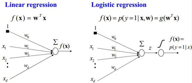

When estimating the parameters of the model, the maximum likelihood estimation method can be used to estimate the parameters of the model, and the logistic regression model can be obtained.
L(w)=log⁡∏i=1N[π(xi)]yi[1−π(xi)]1−yi=∑i=1N[yilog⁡(π(xi))+(1−yi)log⁡(1−π(xi))]=∑i=1N[yilog⁡(π(xi)1−π(xi))+log⁡(1−π(xi))]=∑i=1N[yi(w⋅xi)−log⁡(1+exp⁡(w⋅xi))] \begin{aligned} L(w) =\log \prod_{i=1}^{N}\left[\pi\left(x_{i}\right)\right]^{y_{i}}\left[1-\pi\left(x_{i}\right)\right]^{1-y_{i}} &=\sum_{i=1}^{N}\left[y_{i} \log \left(\pi\left(x_{i}\right)\right)+\left(1-y_{i}\right) \log \left(1-\pi\left(x_{i}\right)\right)\right] \\ &=\sum_{i=1}^{N}\left[y_{i} \log \left(\frac{\pi\left(x_{i}\right)}{1-\pi\left(x_{i}\right)}\right)+\log \left(1-\pi\left(x_{i}\right)\right)\right] \\ &=\sum_{i=1}^{N}\left[y_{i}\left(w \cdot x_{i}\right)-\log \left(1+\exp \left(w \cdot x_{i}\right)\right)\right] \end{aligned} L(w)=logi=1∏N[π(xi)]yi[1−π(xi)]1−yi=i=1∑N[yilog(π(xi))+(1−yi)log(1−π(xi))]=i=1∑N[yilog(1−π(xi)π(xi))+log(1−π(xi))]=i=1∑N[yi(w⋅xi)−log(1+exp(w⋅xi))]
In this way, the problem becomes an optimization problem aiming at the logarithmic likelihood function. By solving the maximum L(w)L(w)L(w)L(w) function, the value of the parameter W can be obtained. Generally, the parameters are updated by the gradient descent method, which is transformed into solving the minimum value.

1.2 LR Multi-Classification Model

1. Logistic regression model is a classification model expressed by the following conditional probability distribution. Logistic regression model can be used for two or more classifications.
P(Y=k∣x)=exp⁡(wk⋅x)1+∑k=1K−1exp⁡(wk⋅x),k=1,2,⋯ ,K−1 P(Y=k | x)=\frac{\exp \left(w_{k} \cdot x\right)}{1+\sum_{k=1}^{K-1} \exp \left(w_{k} \cdot x\right)}, \quad k=1,2, \cdots, K-1 P(Y=k∣x)=1+∑k=1K−1exp(wk⋅x)exp(wk⋅x),k=1,2,⋯,K−1

P(Y=K∣x)=11+∑k=1K−1exp⁡(wk⋅x) P(Y=K | x)=\frac{1}{1+\sum_{k=1}^{K-1} \exp \left(w_{k} \cdot x\right)} P(Y=K∣x)=1+∑k=1K−1exp(wk⋅x)1

Here, xxx is the input feature and www is the weight of the feature.

Logistic regression model is derived from Logistic distribution, and its distribution function F(x)F(x)F(x) F (x) is SSS shape function. Logistic regression model is a logarithmic probability model of output represented by linear function of input.

Code demonstration:

from math import exp
import numpy as np
import pandas as pd
import matplotlib.pyplot as plt
%matplotlib inline
from sklearn.datasets import load_iris
from sklearn.model_selection import train_test_split

class LR_Classifer:
    def __init__(self, max_iter = 200, learning_rate = 0.01):
        self.max_iter = max_iter
        self.learning_rate = learning_rate
        
    def sigmoid(self, x):
        return 1/(1 + exp(-x))
    
    def dat_matrix(self, X):
        data_mat = []
        for d in X:
            data_mat.append([1.0, *d])#Added data to the specified list
            
        return data_mat
    
    def fit(self, X, y):
        data_mat = []
        data_mat = self.dat_matrix(X)
        #print(data_mat)
        #print(len(data_mat[0]))
        self.weights =np.zeros((len(data_mat[0]), 1), dtype=np.float32)
        #print(self.weights)
        for iter_ in range(self.max_iter):
            for i in range(len(X)):
                result = self.sigmoid(np.dot(data_mat[i], self.weights))

                error = y[i] -result

                self.weights += self.learning_rate * error * np.transpose([data_mat[i]])
        print("Result: ", result) 
        print("LR_model(learning rate = {}, max_iter = {})".format(self.learning_rate, self.max_iter))
        
    def score(self, X_test, y_test):
        
        right = 0
        X_test = self.dat_matrix(X_test)
        print(len(X_test))
        for x, y in zip(X_test, y_test):
            result = np.dot(x, self.weights)
            #print(result)
            if (result > 0 and y == 1) or (result < 0 and y == 0):
                right += 1 
        
        return right/len(X_test)
# data
def create_data():
    iris = load_iris()
    df = pd.DataFrame(iris.data, columns=iris.feature_names)
    df['label'] = iris.target
    df.columns = ['sepal length', 'sepal width', 'petal length', 'petal width', 'label']
    data = np.array(df.iloc[:100, [0,1,-1]])
    # print(data)
    return data[:,:2], data[:,-1]

if __name__ == "__main__":
    X, y = create_data()
    X_train, X_test, y_train, y_test = train_test_split(X, y , test_size = 0.3 )
	lr_clf = LR_Classifer()
    lr_clf.fit(X_train, y_train)
    lr_clf.score(X_test, y_test)
    lr_clf.weights

Code results:

Result:  0.9894921837831687
LR_model(learning rate = 0.01, max_iter = 200)
30
array([[-0.90014833],
       [ 3.4473245 ],
       [-5.692265  ]], dtype=float32)

Drawing code:

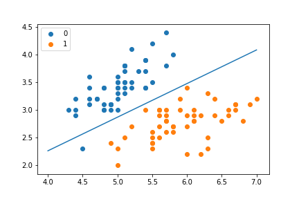
x_points = np.arange(4, 8)
y_ =-(lr_clf.weights[1] * x_points + lr_clf.weights[0])/lr_clf.weights[2]
print(y_)
plt.plot(x_points, y_)

plt.scatter(X[:50, 0],X[:50, 1], label = "0")
plt.scatter(X[50:, 0],X[50:, 1], label = "1")
plt.legend().

Result:

2. Maximum Entropy Model

2.1 Maximum Entropy Principle

Maximum Entropy Principle is a criterion for probabilistic model learning. Maximum Entropy Principle holds that the model with the greatest entropy is the best one among all possible probability models (distributions) when learning probability models. Constraints are usually used to determine the set of probability models, so the maximum Entropy Principle can also be expressed as selecting the model with the greatest entropy in the set of models satisfying constraints. The original text is as follows:

Model all that is known and assume nothing about that which is unknown. In other words, given a collection of facts, choose a model which is consistent with all the facts, but otherwise as uniform as possible.

– Berger, 1996

The maximum entropy principle is summarized as follows:

Equal probability denotes ignorance of facts, since there is no more information, this judgment is reasonable.
Maximum Entropy Principle holds that the probability model to be selected must first satisfy the existing facts, that is, the constraints.
Maximum Entropy Principle Selects Appropriate Probability Model Based on Existing Information (Constraint Conditions)
Maximum Entropy Principle holds that the uncertain parts are equally possible, and equal possibilities are expressed by maximizing the entropy.
Maximum Entropy Principle, Acknowledging Existing and Unbiased to the Unknown
Maximum Entropy Principle does not directly concern feature selection, but feature selection is very important, because constraints may be thousands of.

2.2 Definition of Maximum Entropy Model

Assuming that the classification model is a conditional probability distribution, P(Y X) P(Y X) P(Y X), X < X R nX in mathcal {X} sube mathbf R ^ nX < X Rn, given a training set T={(x1,y1),(x2,y2),... (xN, yN)} T={(x_1, y_1), (x_2, y_2), dots, (x_N, y_N)} T={(x1, y1), (x_2, y_2),... (xN, yN)}

NNN is the training sample size. The empirical distributions of joint distribution P(x,Y)P(X,Y)P(X,Y)P(X,Y) and edge distribution P(X) are P~(x)widetilde P(x,Y) and P(x)widetilde P(x,Y) and P(x)widetilde P(x,Y) respectively.

P~(X=x,Y=y)=ν(X=x,Y=y)NP~(X=x)=ν(X=x)N \begin{aligned} &\widetilde P (X=x, Y=y)=\frac{\nu(X=x, Y=y)}{N} \\ &\widetilde P (X=x)=\frac {\nu (X=x)}{N} \end{aligned} P(X=x,Y=y)=Nν(X=x,Y=y)P(X=x)=Nν(X=x)
The above two are different data samples, the proportion in the training data set.

If nnn eigenfunctions are added, nnn constraints can be added, and a column of features can be added.

Suppose that the set of models satisfying all constraints is $\mathcal {C} \equiv\{{P\\\mathcal {P} | E_P (f_i) = E {\widetilde {P} {P}(f_i) {(f_i) {, I = 1,2, \\dots, n}} & font&lt&gt, lt, defined in the conditional probability distribution; / font&font&font; / font&font&font;; / font&font>>Conditional Entropy Defined on Conditional Probability Distribution P(Y|X) If the conditional entropy above is H=- sum limits {x, y} widetilde {P} (x) P (y | x) log {P (y | x)}, then the model set of conditional entropy in the conditional entropy of the model set cal {C} is called the maximum entropy model, and the logarithm in the formula above is natural logarithm. The model with the largest characteristic function is called the maximum entropy model, and the logarithm in the formula above is natural logarithm. The model with the largest characteristic function is called the maximum entropy model, and the logarithm in the formula above is natural logarithm. The expected value of the eigenfunction f(x,y) with respect to empirical distribution with respect to the expected value of empirical distributionwidetilde P(X,Y) is expressed by E {widetilde P}(f)$.

EP~(f)=∑x,yP~(x,y)f(x,y) E_{\widetilde P}(f)=\sum\limits_{x,y}\widetilde P(x,y)f(x,y) EP(f)=x,y∑P(x,y)f(x,y)
The expected values of the characteristic function f(x,y)f(x,y)f(x,y) f (x, y) on the model P(Y X) P(Y X) P(Y X) and the empirical distribution P (X) widetilde P (X) P (X) P (X) are expressed by EP (f) E {P} (f) EP f).

EP(f)=∑x,yP~(x)P(y∣x)f(x,y) E_{P}(f)=\sum\limits_{x,y}{\widetilde P(x)P(y|x)f(x,y)} EP(f)=x,y∑P(x)P(y∣x)f(x,y)

If the model can get information from training data, then there is
P~(x,y)=P(y∣x)P~(x) \widetilde{P}(x,y)=P(y|x)\widetilde{P}(x) P(x,y)=P(y∣x)P(x)
It can be assumed that the two expectations are equal, i.e.

EP(f)=EP~(f)E_P(f)=E_{\widetilde P}(f)EP(f)=EP(f)

The above one is also a constraint equation.

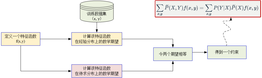
The empirical distribution of joint distribution and edge distribution can be obtained by analyzing the data of known training sets. Characteristic functions are used to describe a fact between input x x x and output y y y of f(x,y)f(x, y)f(x,y).

f(x,y)={1x and y satisfy a fact 0 otherwise f(x,y) = \begin{cases} 1 & amp; X and y satisfy a fact\ 0 & amp; otherwise \end{cases} f(x,y)={10 X and y satisfy a fact otherwise

Constitution of constraints:

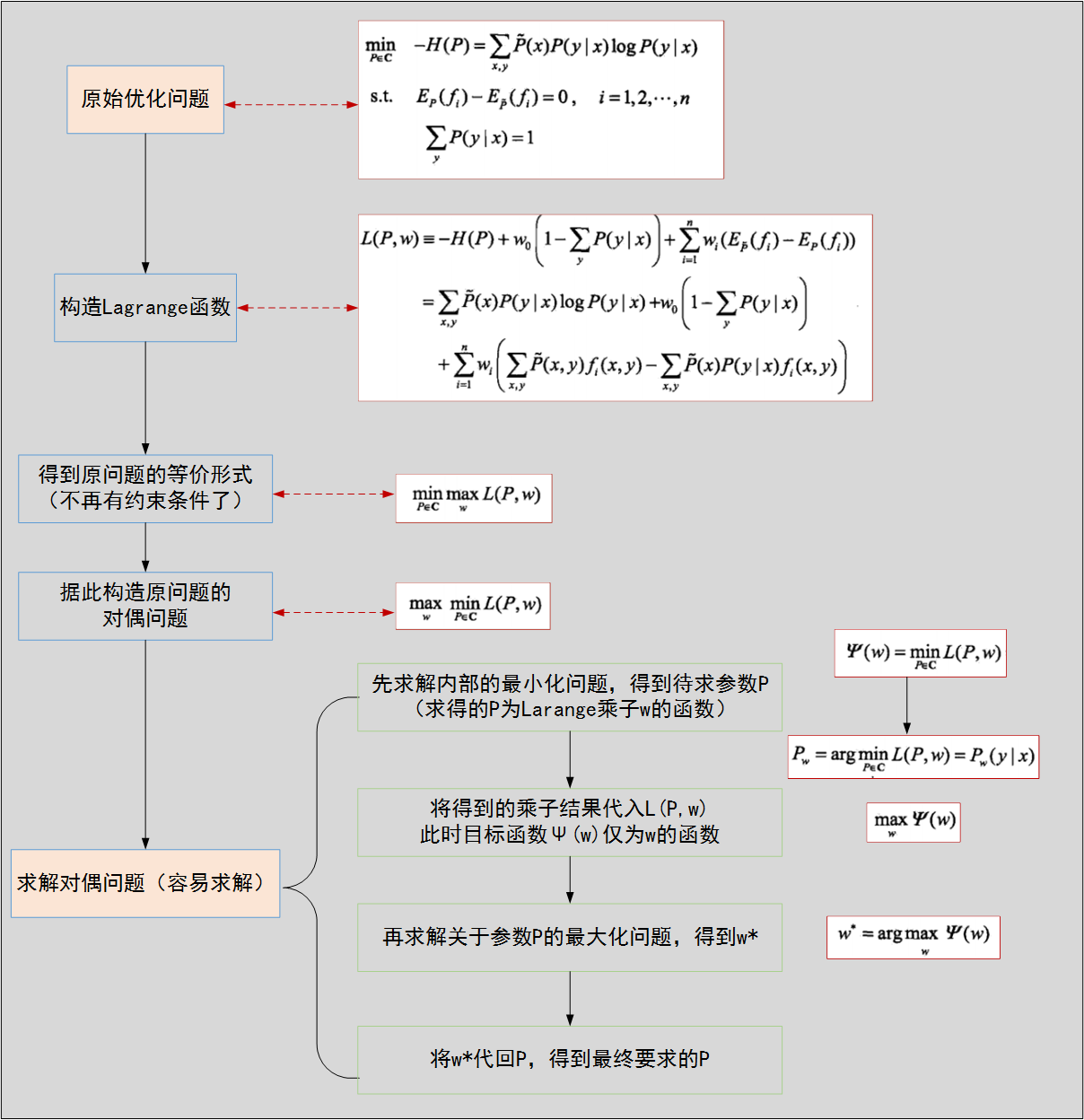
Maximum Entropy Estimation Model Algorithms: