1. Preparatory knowledge

1.1 filtering, kernel and convolution

• The filter is an algorithm for calculating a new image I '(x,y) from an image I(x,y) according to the region near the pixel x,y. The template specifies the shape of the filter and the composition law of the values of pixels in this area, also known as "filter" or "core".

1.2 boundary extrapolation and boundary treatment

• The output image obtained by filtering operations in OpenCV (such as cv::blur(), cv::erode(), cv::dilate(), etc.) is the same shape as the source image. In order to achieve this effect, OpenCV uses the method of adding virtual pixels around the source image** cv::blur() * * function realizes the average operation of each pixel and surrounding pixels of the image.

1.2.1 custom border

• When processing an image, as long as you tell the called function the rule of adding virtual pixels, the library function and automatically create virtual pixels. Similarly, in order to clarify the intention of an operation, we should pay attention to the method used by the function when creating virtual pixels.
• CV:: copymaker border() is a function to create a border for an image. By formulating two images, the first is the source image and the second is the expanded image. At the same time, the filling method is well-known. This function will save the filled results of the first image in the second image.

	void copyMakeBorder(
		InputArray src, 
		OutputArray dst,
		int top, 
		int bottom,
		int left, 
		int right,
		int borderType, //How pixels are filled
		const Scalar& value = Scalar()
		);

• Boundary type

Border type	effect
cv::BORDER_CONSTANT	Copies the specified constant extension boundary
cv::BORDER_WRAP	Copy the pixel extension boundary of the opposite edge
cv::BORDER_REPLICATE	Copy the pixel extension boundary of the edge
cv::BORDER_REFLECT	Extend boundaries by mirroring
cv::BORDER_REFLECT_101	Copy extended boundaries by mirroring, except boundary pixels
cv::BORDER_DEFAULT	The default is CV:: border_ REFLECT_ one hundred and one

1.2.2 user defined extrapolation

• In some cases, we need to calculate the position of the pixel referenced by a particular pixel. For example, given an image with width w and height h, we need to know which pixel is assigned to the virtual pixel * * (w+dx,h+dy) * *. The function to calculate the result is CV:: borderinterplate()

	int borderInterpolate(
		int p, //coordinate
		int len, //Length (the actual size of the image in the associated direction)
		int borderType //Boundary type
		);

• cv::borderInterpolate() calculates the extrapolation on one dimension at a time. For example, we can calculate the value of a specific pixel under mixed boundary conditions and use * * CV:: border in one dimension_ REFLECT_ 101, use CV:: border in another dimension_ Wrap style * *.

	float val = img.at<float>(
		cv::borderInterpolate(100, img.rows, BORDER_REFLECT_101),
		cv::borderInterpolate(100, img.rows, BORDER_WRAP)
		);

• Inside OpenCV, this is a frequently used function, such as cv::copyMakeBorder, or you can call this function in a custom algorithm.

2. Thresholding operation

2.1 threshold

2.1.1 function introduction

• According to personal preference, the thresholding operation can be understood as an operation with 1 × 1, and perform a linear operation on each pixel.

	double threshold(
		InputArray src, 
		OutputArray dst,
		double thresh, //threshold
		double maxval, //Maximum value given
		int type  //Operation type
		);

Threshold type	operation
cv::THRESH_BINARY	DST=(SRC>thresh)?MAXVALUE:0
cv::THRESH_BINARY_INV	DST=(SRC>thresh)?0:MAXVALUE
cv::THRESH_TRUNC	DST=(SRC>thresh)?THRESH:SRC
cv::THRESH_TOZERO	DST=(SRC>thresh)?SRC:0
cv::THRESH_TOZERO_INV	DST=(SRC>thresh)?0:SRC

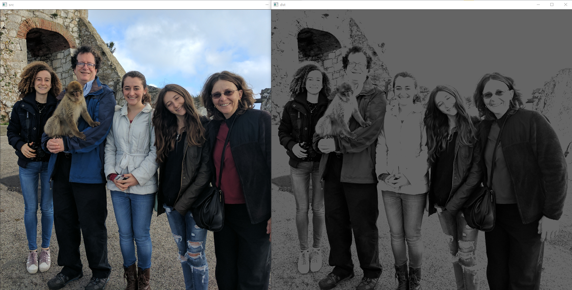
2.1.2 routine 10-1 image addition and thresholding operation

// Example10_1.cpp: defines the entry point of the console application.
//

#include "stdafx.h"
#include <opencv2\opencv.hpp>
#include <iostream>
using namespace cv;
using namespace std;

/**********
	Add the three channels of an image and limit the pixel value to 100
**/

void sum_rgb(const Mat& src, Mat& dst) 
{
	vector<Mat> planes;
	split(src, planes);
	Mat b = planes[0], g = planes[1], r = planes[2], s;

	//We did not add the data directly and store it in an 8-bit array (this may cause out of bounds)
	//Instead, the three channels are added after taking the same weight value, and then the value greater than 100 is truncated
	addWeighted(r, 1. / 3, g, 1. / 3, 0.0, s);
	addWeighted(s, 1., b, 1. / 3, 0.0, s);
	
	threshold(s, dst, 100, 100, THRESH_TRUNC);
}

/*****************
	Alternative methods for combining and thresholding image planes
*/
void sum_rgb2(const Mat& src, Mat& dst)
{
	vector<Mat> planes;
	split(src, planes);
	Mat b = planes[0], g = planes[1], r = planes[2];

	// Accumulate can accumulate an 8-bit integer image into a floating-point image
	Mat s = Mat::zeros(b.size(), CV_32F);
	accumulate(b, s);
	accumulate(g, s);
	accumulate(r, s);
	
	threshold(src, s, 100, 100, THRESH_TRUNC);
	s.convertTo(dst, b.type());
}

int main()
{
	Mat src = imread("./faces.png"), dst;
	if (src.empty())
		cout << "Unable to open image" << endl;

	sum_rgb(src, dst);
	imshow("src", src);
	imshow("dst", dst);

	Mat dst2;
	sum_rgb(src, dst2);
	imshow("dst2", dst2);

	waitKey(0);
    return 0;
}

2.2 Otsu algorithm

• threshold() can also automatically determine the optimal threshold. You only need to pass the value CV:: threshold to the parameter threshold_ Otsu is enough.
• OTSU algorithm is to traverse all possible thresholds, and then calculate the variance of the two types of pixels of each threshold result (that is, the two types of pixels below and above the threshold).
• This method takes the same time whether it is the minimum variance or the maximum variance. The reason is that you need to traverse all possible thresholds, which is not a relatively efficient process.

2.3 adaptive threshold

2.3.1 adaptiveThreshold()

	void adaptiveThreshold(
		InputArray src, 
		OutputArray dst,
		double maxValue, //Maximum
		int adaptiveMethod, //Two best fit threshold methods are supported
		int thresholdType, //Operation type
		int blockSize,  
		double C
		);

• The following two methods calculate the adaptive threshold T(x,y) of Zhuge pixels by calculating the b around each pixel position × The weighted average of the b region and then subtract the constant C, where b is given by blockSize.
• cv::ADAPTIVE_THRESH_MEAN_C. When the mean value is obtained, the weight is to be equal;
• cv::ADAPTIVE_THRESH_GAUSSIAN_C. (x,y) the weight of the surrounding pixels is obtained by Gaussian equation according to the distance from the center point;
• The threshold changes automatically throughout the process
• Adaptive threshold is very effective when there is a large light and dark difference in the image.
• This function only processes single channel 8-bit or floating-point images, and requires that the source image and target image are different.

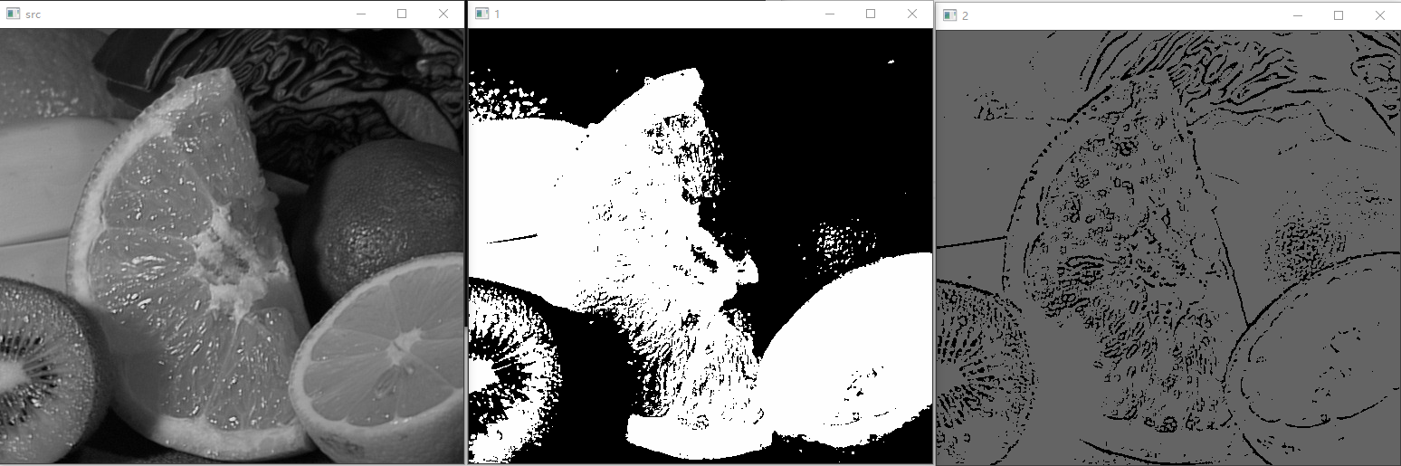
2.3.2 routine 10-3 adaptive threshold code

// Example10_3.cpp: define the entry point of the console application.
//

#include "stdafx.h"
#include <opencv2\opencv.hpp>
using namespace cv;

int main()
{
	Mat srcImage = imread("./fruits.jpg", IMREAD_GRAYSCALE);
	Mat mat1, mat2;
	threshold(srcImage, mat1, 100, 254, THRESH_BINARY);
	adaptiveThreshold(srcImage, mat2, 100, ADAPTIVE_THRESH_GAUSSIAN_C, THRESH_BINARY, 15, 10);
	imshow("src", srcImage);
	imshow("1", mat1);
	imshow("2", mat2);

	waitKey(0);
    return 0;
}

3. Smooth

• The purpose of smoothing image is usually to reduce noise and artifacts. Smoothing is also very important when reducing resolution.

3.1 simple fuzzy and block filters

3.1.1 simple fuzzy

	void blur(
		InputArray src, 
		OutputArray dst,
		Size ksize,  
		Point anchor = Point(-1, -1), 
		int borderType = BORDER_DEFAULT //Smoothing method of edge pixels
		);

• blur() realizes simple blur. Each value in the target image is the average value of pixels in a core at the corresponding position in the source image.
• ksize: kernel size.
• anchor: Specifies the alignment between the core and the source image during calculation. The default is cv::Point(-1,-1), indicating that the core is centered relative to the filter.
• If the source image is a multi-channel image, each channel is calculated separately.

3.1.2 block filter

	void boxFilter(
		InputArray src,
		OutputArray dst,
		int ddepth,
		Size ksize,
		Point anchor = Point(-1, -1),
		bool normalize = true,  //Normalized
		int borderType = BORDER_DEFAULT
		);

• The block filter is rectangular, and all values K in the filter are equal.
• Generally, all values K are 1 or 1/A, and a is the area of the filter. When it is 1/A, it is called normalized block filter.
• boxFilter() is a generalized form, while blur() is a specialized form.
• The fundamental difference between the two is that the former can be called in the form of normalization, and the output image depth can be controlled (* * blur() * * the output depth is consistent with the source image).
• If the variable ddepth is set to - 1, the depth of the target image will be consistent with the source image; Otherwise, it can be set to any other depth, such as CV_32F

3.2 median filter

	void medianBlur(
		InputArray src,
		OutputArray dst, 
		int ksize
		);

• The median filter replaces each pixel with a median or "median" pixel (relative to the average pixel) in the rectangular neighborhood surrounding the pixel.
• Median filtering is very sensitive to large isolated outliers (such as shooting noise in digital images).
• A small number of points with large deviation will also seriously affect the mean filter, and the median filter can eliminate the influence of outliers by taking the middle point.
• Median filter is a nonlinear kernel.

3.3 Gaussian filter

void GaussianBlur(
	InputArray src, 
	OutputArray dst,
	Size ksize,
	double sigmaX,
	double sigmaY = 0,
	int borderType = BORDER_DEFAULT
	);

• Gaussian filter is the most useful filter. It performs normalized Gaussian kernel filtering on the input array, and then outputs the target array.
• For Gaussian filters, ksize specifies the width and height of the filter core, and sigma X represents the Sigma value of the Gaussian core in the X direction. If only x is given and Y is set to 0, then y will be equal to X;
• OpenCV provides performance optimization for commonly used kernels. three × 3,5 × 5,7 × The standard sigma core of 7 (sigma x = 0) has better performance than other cores.

3.4 bilateral filter

	void bilateralFilter(
		InputArray src, 
		OutputArray dst,
		int d, //The diameter of pixel neighborhood has a great impact on the efficiency of the algorithm. Generally, video processing does not exceed 5. You can set it to - 1, and the function will automatically design the amount of sigma space for the image
		double sigmaColor,  //The Sigma value and sigmaColor of the color space filter are similar to the parameter sigma in the Gaussian filter
		double sigmaSpace, //The Sigma value of the filter in the coordinate space is sigma space. The greater the sigmaColor, the greater the intensity (color) included in the smoothing
		int borderType = BORDER_DEFAULT
		);

• Bilateral filter is a relatively large image analysis operator, that is, the edge is kept smooth.
• The process of Gaussian blur is to slow down the change of pixels in space, so it is closely related to the neighborhood, and the change range of random noise among pixels will be very large (that is, the noise is not spatially related). Based on this premise, Gaussian smoothing can reduce the noise and retain the small signal. However, this method destroys the edge information, and the final result is that Gaussian blur blurs the edge.
• Similar to Gaussian smoothing, bilateral filtering weighted average each pixel and the pixels in its region. Its weight consists of two parts: the first part is the same as Gaussian smoothing; The second part is also Gaussian weight. The difference is that it is not calculated based on spatial distance, but the color intensity difference. On the channel (color) image, the intensity difference is replaced by the weighted accumulation of each component.
• Bilateral filtering can be regarded as Gaussian smoothing, but pixels with higher similarity have higher weight, more obvious edge and higher contrast. The effect of bilateral filtering is to turn the source image into a watercolor painting. This idea is more significant after many iterations. Therefore, this method is very useful in the field of image segmentation.

4. Derivative and gradient

4.1 Sobel derivative

	void Sobel(
		InputArray src, 
		OutputArray dst, 
		int ddepth, //The depth or type of the target image. For example, if src is an 8-bit image, dst needs at least cv_ The 16S depth guarantees no overflow
		int dx, //The derivation order 0 means no derivation in this direction
		int dy, //The derivation order 0 means no derivation in this direction
		int ksize = 3, //Odd number > 1 means the width and height of the called filter. At present, the maximum support is 31
		double scale = 1, //Scaling factor  
		double delta = 0, //Offset factor   
		int borderType = BORDER_DEFAULT
		);

• The most commonly used operator to represent differential is Sobel, which can realize arbitrary order derivative and mixed partial derivative.
• One advantage of Sobel operator is that the kernel can be defined as various sizes, and these kernels can be constructed quickly and iteratively.
• A large kernel can better approximate the derivative because it can eliminate the influence of noise. however. If the derivative changes sharply in space, the result will be biased.
• Sobel is not a real derivative because it is defined in discrete space. It is actually a polynomial. The second-order Sobel operation in the x direction represents not the second derivative, but the local fitting of the parabolic function. This also explains why a larger core is used, and a larger core fits more pixels.

4.2 Scharr filtering

• The disadvantage of Sobel operator is that the accuracy is not high when the kernel is small. For large kernels, the approximation process uses more points, so the accuracy problem is not significant.
• For 3 × 3, the farther the gradient angle is from the horizontal or vertical direction, the more obvious the error is.
• When Sobel is called, set ksize to cv::SCHARR to eliminate 3 × 3 the error caused by such a small but fast Sobel derivative filter. Scharr is also fast, but with higher accuracy.

4.3 Laplace transform

	void Laplacian(
		InputArray src,
		OutputArray dst, 
		int ddepth,
		int ksize = 1, 
		double scale = 1,
		double delta = 0,
		int borderType = BORDER_DEFAULT
		);

• Laplacian() can be used for various scene processing. A common application is matching spots.
• Laplacian() is the sum of the derivatives of the image in the X and Y axes, which means that the value at a surrounded point or small spot (smaller than ksize) will become large. On the contrary, the value at points surrounded by smaller values or small spots will become large in the negative direction.
• Therefore, Laplacian can also be used for edge detection.

5. Image morphology

5.1 corrosion and expansion

5.2 general morphological function

5.3 open and close operations

5.4 morphological gradient

5.5 top hat and black hat

5.6 custom core

6. Convolution with any linear filter

6.1 convolution with cv::filter2D()

6.2 using separable cores via cv::sepFilter2D

6.3 generating convolution kernel