This picture and text is the learning notes of Datawhale team learning pytoch. The main contents include the concept of tensor (0-dimensional, 1-dimensional, 2-dimensional, 3-dimensional, 4-dimensional tensor, etc.), the principle of automatic derivation (understanding through dynamic graph), and the understanding of parallelism.

Chapter 02 pytoch Basics

2.1 tensor

In this chapter, we begin to introduce the basic knowledge of PyTorch. We start with tensor, establish the description of data, then introduce the operation of tensor, and finally talk about the core package of all neural networks in PyTorch, autograd, that is, automatic differentiation. After understanding these contents, we can better understand PyTorch code. Now let's start ~

brief introduction

The tensor defined in geometric algebra is a generalization based on scalar, vector and matrix. For example, scalar can be regarded as 0-dimensional tensor, vector can be regarded as 1-dimensional tensor, and matrix is 2-dimensional tensor.

• 0-dimensional tensor / scalar: scalar is a number. Such as 1.
• 1D tensor / vector: e.g. [1,2,3].
• 2-dimensional tensor / matrix: such as [[1,2,3], [4,5,6]].
• Three dimensional tensor: such as [[[1, 4, 7], [2, 5, 8]], [[1, 2, 3], [4, 5, 6]].

Tensor is the basis of modern machine learning. Its core is a data container. In most cases, it contains numbers and sometimes strings, but this is rare. So think of it as a digital bucket.

The data used in machine learning (deep learning), including structural data (data table, sequence) and non structural data (picture, video) are tensors, which are summarized as follows:

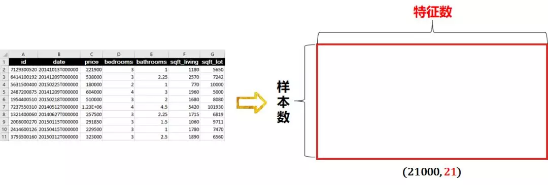
• Data table: 2D, shape = (number of samples, number of features)
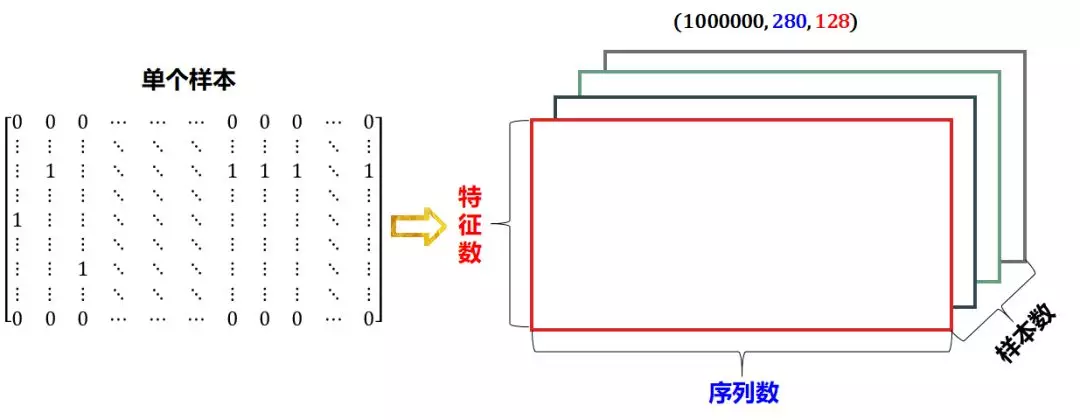
• Sequence class: 3D, shape = (number of samples, step size, number of features)
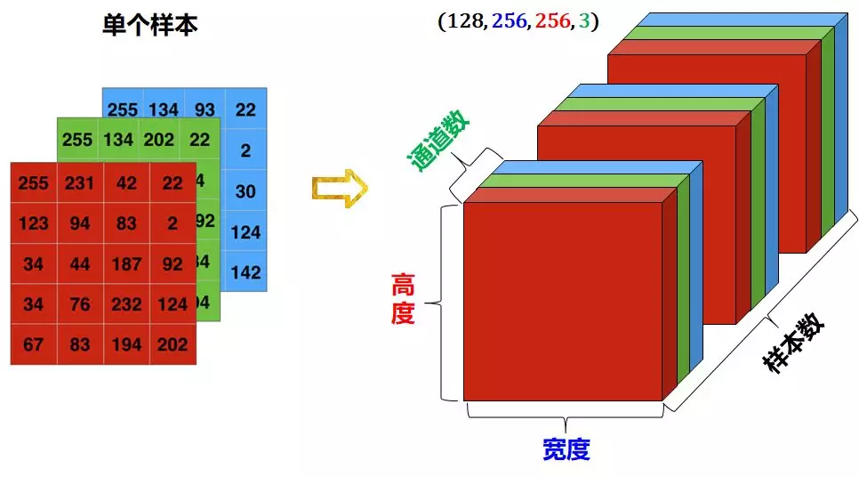
• Image class: 4D, shape = (number of samples, width, height, number of channels)
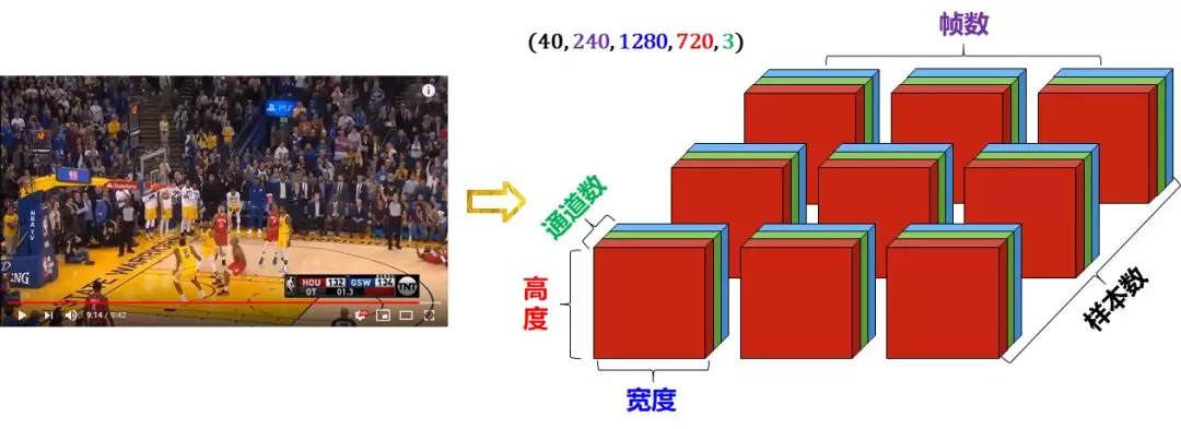
• Video class: 5D, shape = (number of samples, number of frames, width, height, number of channels)

Machine learning, especially deep learning, requires a lot of data, so the number of samples must account for one dimension. Conventionally, we call it dimension 1. In this way, the tensor to be processed by machine learning starts from at least 2 dimensions.

Two dimensional tensors are matrices, also known as data tables, which are generally stored in csv.

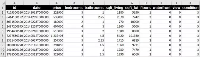
This set of table contains 21000 data, including 21 columns: its price (y), square feet, number of bedrooms, floor, date, renovation year, etc. The data shape is (21000, 21). The linear regression of traditional machine learning can predict house prices.

The data representation of two-dimensional tensor is as follows:

3D sequence data

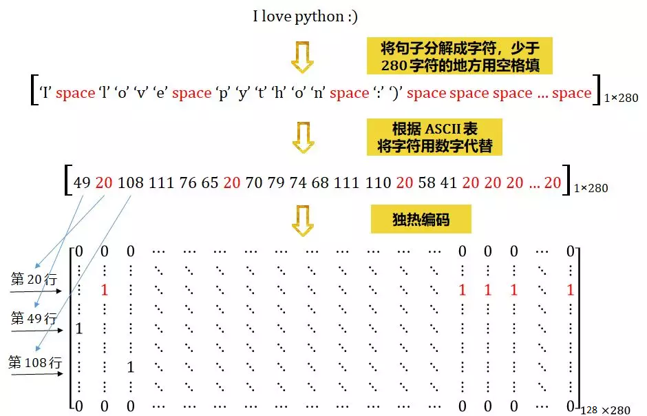
Each tweet on Twitter is limited to 280 characters. When encoding tweets, the 280 character sequence is one hot encoded into an ASCII table containing 128 characters, as shown below.

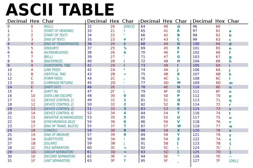
In this way, each tweet can be encoded as a two-dimensional tensor, shape (280, 128). For example, a tweet is "I love python" 😃”， This sentence is mapped to the ASCII table and becomes:

If 1 million tweets are collected, the shape of the whole data set is (1000000, 280, 128). The pairwise regression of traditional machine learning can be used for emotion analysis.

The data representation of 3D tensor is as follows:

? - 3D = time series common data is stored in tensor time series data and stock price text data

4D image data

Images usually have three dimensions: width, height and color channel. Although black-and-white images (such as MNIST numbers) have only one color channel, according to convention, we still regard it as three dimensions, that is, the color channel has only one dimension.

• A set of black-and-white photos can be stored as a 4-dimensional tensor with a shape of (number of samples, width, height, 1)
• A set of color photos can be stored as a 4-dimensional tensor with the shape of (number of samples, width, height, 3)

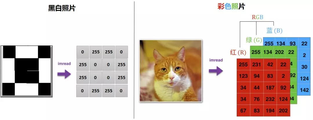
Usually 0 represents black and 255 represents white.

The data representation of 4-dimensional tensor is as follows:

5D video data

Video can be decomposed into frames.

• Each frame is a color image and can be stored in a 3D tensor with a shape of (width, height, channel)
• The video screen (a sequence of frames) can be stored in a 4D tensor whose shape is (number of frames, width, height, channel)
• A batch of different videos can be stored in a 5D tensor whose shape is (number of samples, number of frames, width, height, channel)

The following 9:42 second 1280x720 YouTube Video (harden's three-point kill warrior) is decomposed into 40 sample data, each sample includes 240 frames. Such video clips will be stored in tensors with shapes of (40, 240, 1280, 720, 3).

The data representation of 5-Dimensional tensor is as follows:

Tensors can be regarded as multidimensional arrays. Let's use Python's numpy to define tensors.

import numpy as np

# 0-dimensional tensor ()
x0 = np.array(28)

# 1D tensor (3,)
x1 = np.array([1,2,3])

# 2-dimensional tensor (2, 3)
x2=np.array([[1,2,3],[4,5,6]])

# Three dimensional tensor (3, 3, 4)
x3 = np.array([[[1, 4, 7, 3], [2, 5, 8, 5], [3, 6, 9, 4]],
               [[1, 2, 3, 4], [4, 5, 6, 3], [7, 8, 9, 5]],
               [[9, 8, 7, 5], [6, 5, 4, 4], [3, 2, 1, 3]]])

# 4-dimensional tensor (2, 5, 4, 3)
x4 = np.ones((2,5,4,3))

It is not difficult to see:

• X0, x1, X2 and X3 are defined by the elements in the tensor directly set by np.array.
• X4 defines a tensor in which all elements are 1 by np.ones and the shape of the tensor (2,5,4,3)

In PyTorch, torch.Tensor is the main tool for storing and transforming data. If you have used NumPy before, you will find that Tensor and NumPy's multidimensional arrays are very similar. However, Tensor provides more functions such as GPU calculation and automatic gradient calculation, which makes Tensor a data type more suitable for deep learning.

from __future__ import print_function
import torch

Tensor operation mainly includes tensor structure operation and tensor mathematical operation operation.

• Tensor's structural operations include: creating tensors, viewing attributes, modifying shapes, specifying devices, data conversion, index slicing, broadcasting mechanism, element operation, merging operation;
• Tensor's mathematical operations include scalar operation, vector operation, matrix operation and comparison operation;

Create tensor

# (0-dimensional tensor)

x = torch.tensor(2)
print(x, x.shape, x.type())
# tensor(2) torch.Size([]) torch.LongTensor

y = torch.Tensor(2)
print(y, y.shape, y.type())
# tensor([0., 0.]) torch.Size([2]) torch.FloatTensor

Note that there is no difference between torch.tensor and torch.tensor, but the results are very different.

• torch.tensor(2) returns constant 2. The data type is inferred from the data, where 2 represents the data value.
• torch.Tensor(2) uses the global default dtype (FloatTensor) to return a vector with size 2 and the initial value is 0;

Directly use the data to construct a tensor:

# 1-dimensional tensor

x = torch.tensor([5.5, 3])
print(x, x.shape, x.type())

# tensor([5.5000, 3.0000]) torch.Size([2]) torch.FloatTensor

Construct a randomly initialized matrix:

# 2D vector

torch.manual_seed(20211013)
x = torch.rand([4, 3])
print(x, x.shape, x.type())

# tensor([[0.4786, 0.4584, 0.2201],
#         [0.5064, 0.5879, 0.9110],
#         [0.8603, 0.5285, 0.0871],
#         [0.8849, 0.4521, 0.3099]]) torch.Size([4, 3]) torch.FloatTensor

Construct a matrix with all 0 and the data type is long.

# 2D vector

x = torch.zeros([4,3],dtype=torch.long)
print(x)

# tensor([[0, 0, 0],
#         [0, 0, 0],
#         [0, 0, 0],
#         [0, 0, 0]])

Create a tensor based on the existing tensor:

x = torch.tensor([5.5, 3])
x = x.new_ones([4,3])
print(x,x.type())

# tensor([[1., 1., 1.],
#         [1., 1., 1.],
#         [1., 1., 1.],
#         [1., 1., 1.]], dtype=torch.float64)

# Create a new tensor, and the returned tensor has the same torch.dtype and torch.device by default
# You can also write x = torch.ones(4, 3, dtype=torch.double) as before

x = torch.ones([4,3],dtype=torch.double)
print(x)

# tensor([[1., 1., 1.],
#         [1., 1., 1.],
#         [1., 1., 1.],
#         [1., 1., 1.]], dtype=torch.float64)

x = torch.rand_like(x,dtype=torch.float)
# Reset data type

print(x)
# The result will be the same
# tensor([[0.5162, 0.1575, 0.3045],
#         [0.8349, 0.5412, 0.5001],
#         [0.8255, 0.7037, 0.3061],
#         [0.4699, 0.6661, 0.0216]])

Get its dimension and other attribute information:

• tensor.shape, tensor.size(): returns the shape of tensor;
• tensor.ndim: view the dimension of tensor;
• tensor.dtype, tensor.type(): view the data type of tensor;
• tensor.is_cuda: check whether the tensor is on the GPU;
• tensor.grad: view the gradient of tensor;
• tensor.requires_grad: see if the tensor is differentiable.

torch.manual_seed(20211013)
x = torch.rand([4, 3])
print("shape: ", x.shape, x.size())
print("dimension: ", x.ndim)
print("type: ", x.dtype, x.type())
print("cuda: ", x.is_cuda)
print("gradient: ", x.grad)
print("Is it differentiable: ", x.requires_grad)

# Shape: torch.Size([4, 3]) torch.Size([4, 3])
# Dimension: 2
# Type: torch.float32 torch.FloatTensor
# cuda:  False
# Gradient: None
# Differentiability: False

There are also some common functions for constructing Tensor:

function	function
Tensor(*sizes)	Base constructor. Construct a tensor directly from the parameters, and support List and Numpy arrays.
tensor(data)	Similar to np.array
ones(*sizes)	Specify shape to generate data of all 1 elements.
zeros(*sizes)	Specify a shape to generate data with all 0 elements.
eye(*sizes)	The diagonal is 1 and the rest is 0. Specify the number of (rows and columns) to create a two-dimensional unit Tensor.
arange(s,e,step)	From s to e, step generates a sequence tensor for step.
linspace(s,e,steps)	From s to e, it is evenly divided into step parts.
logspace(s,e,steps)	From 10^s to 10^e, evenly divide into steps.
rand/randn(*sizes)	Generate [0,1] uniform distribution and standard normal distribution data.
normal(mean,std)/uniform(from,to)	Normal distribution / uniform distribution
randperm(m)	Random arrangement

operation

Some addition operations:

torch.manual_seed(20211013)
x = torch.rand([4, 3])
y = torch.ones([4, 3])
print(x)
# tensor([[0.4786, 0.4584, 0.2201],
#         [0.5064, 0.5879, 0.9110],
#         [0.8603, 0.5285, 0.0871],
#         [0.8849, 0.4521, 0.3099]])

# Mode 1
print(x + y)
# tensor([[1.4786, 1.4584, 1.2201],
#         [1.5064, 1.5879, 1.9110],
#         [1.8603, 1.5285, 1.0871],
#         [1.8849, 1.4521, 1.3099]])

# Mode 2
print(torch.add(x, y))
# tensor([[1.4786, 1.4584, 1.2201],
#         [1.5064, 1.5879, 1.9110],
#         [1.8603, 1.5285, 1.0871],
#         [1.8849, 1.4521, 1.3099]])

# Mode 3 provides an output tensor as a parameter
result = torch.empty([4, 3])
torch.add(x, y, out=result)
print(result)
# tensor([[1.4786, 1.4584, 1.2201],
#         [1.5064, 1.5879, 1.9110],
#         [1.8603, 1.5285, 1.0871],
#         [1.8849, 1.4521, 1.3099]])

# Mode 4 in place
y.add_(x)
print(y)
# tensor([[1.4786, 1.4584, 1.2201],
#         [1.5064, 1.5879, 1.9110],
#         [1.8603, 1.5285, 1.0871],
#         [1.8849, 1.4521, 1.3099]])

Index operation: (similar to numpy)

It should be noted that the indexed results share memory with the original data, that is, if one is modified, the other will be modified.

torch.manual_seed(20211013)
x = torch.rand([4, 3])
print(x)
# tensor([[0.4786, 0.4584, 0.2201],
#         [0.5064, 0.5879, 0.9110],
#         [0.8603, 0.5285, 0.0871],
#         [0.8849, 0.4521, 0.3099]])

# Take the second column
print(x[:, 1])
# tensor([0.4584, 0.5879, 0.5285, 0.4521])

y = x[0, :]
y += 1
print(y)
# tensor([1.4786, 1.4584, 1.2201])

print(x[0, :])
# tensor([1.4786, 1.4584, 1.2201]) # The source tensor has also been changed

Change size: if you want to change the size or shape of a tensor, you can use torch.view:

torch.manual_seed(20211013)
x = torch.randn([4, 4])
print(x)
# tensor([[ 0.9747,  0.8300, -0.6734, -0.4365],
#         [ 0.1867,  0.9543,  0.3457, -0.1776],
#         [ 0.5936, -0.7330,  0.2092,  1.1053],
#         [ 1.3183, -1.9817,  1.9537, -1.2133]])

y = x.view(16)
z = x.view(-1, 8) # -1 means that the dimension of this dimension is determined by other dimensions
print(x.size(), y.size(), z.size())
# torch.Size([4, 4]) torch.Size([16]) torch.Size([2, 8])

print(y)
# tensor([ 0.9747,  0.8300, -0.6734, -0.4365,  0.1867,  0.9543,  0.3457, -0.1776,
#          0.5936, -0.7330,  0.2092,  1.1053,  1.3183, -1.9817,  1.9537, -1.2133])

print(z)
# tensor([[ 0.9747,  0.8300, -0.6734, -0.4365,  0.1867,  0.9543,  0.3457, -0.1776],
#         [ 0.5936, -0.7330,  0.2092,  1.1053,  1.3183, -1.9817,  1.9537, -1.2133]])

Note that the new tensor returned by view() shares memory with the source tensor (in fact, it is the same tensor), that is, change one of them, and the other will change accordingly. As the name suggests, view only changes the degree of observation of this tensor.

x += 1
print(x)
# tensor([[ 1.9747,  1.8300,  0.3266,  0.5635],
#         [ 1.1867,  1.9543,  1.3457,  0.8224],
#         [ 1.5936,  0.2670,  1.2092,  2.1053],
#         [ 2.3183, -0.9817,  2.9537, -0.2133]])

print(y) # Also added 1
# tensor([ 1.9747,  1.8300,  0.3266,  0.5635,  1.1867,  1.9543,  1.3457,  0.8224,
#          1.5936,  0.2670,  1.2092,  2.1053,  2.3183, -0.9817,  2.9537, -0.2133])

So what if we want to return a really new copy (i.e. no shared memory)?

Pytorch also provides a reshape() function that can change the shape, but this function does not guarantee that it will return a copy, so it is not recommended. It is recommended to create a copy with clone before using view.

Note: another advantage of using clone is that it will be recorded in the calculation diagram, that is, when the gradient is returned to the copy, it will also be transferred to the source Tensor.

If you have an element tensor, use. item() to get the value, which is the scalar of Python:

x = torch.randn(1)
print(x)
# tensor([0.1032])
print(x.item())
# 0.10324124991893768

Tensor in PyTorch supports more than 100 operations, including transpose, index, slice, mathematical operation, linear algebra, random number, etc. Please refer to the official documents.

Broadcasting mechanism

When two tensors with different shapes are calculated by elements, the broadcasting mechanism may be triggered: copy the elements appropriately to make the two tensors have the same shape, and then operate by elements.

import torch

x = torch.arange(1, 3).view(1, 2)
print(x)
# tensor([1, 2])

y = torch.arange(1, 4).view(3, 1)
print(y)
# tensor([[1],
#         [2],
#         [3]])

print(x + y)
# tensor([[2, 3],
#         [3, 4],
#         [4, 5]])

Since X and y are matrices with one row, two columns and three rows and one column respectively, if x + y is to be calculated, the two elements in the first row of X are broadcast (copied) to the second row and the third row, and the three elements in the first column of Y are broadcast (copied) to the second column. In this way, two matrices with three rows and two columns can be added by elements.

2.2 automatic derivation

In PyTorch, the core of all neural networks is autograd package. The autograd package provides an automatic derivation mechanism for all operations on tensors. It is a framework defined by run, which means that back propagation is determined according to how the code runs, and each iteration can be different.

torch.Tensor is the core class of this package. If its property. Requires is set_ grad is True, then it will track all operations on the tensor. When the calculation is completed, all gradients can be calculated automatically by calling. backward(). All gradients of this tensor will be automatically added to the. grad attribute.

Note: in y.backward(), if y is a scalar, no parameters need to be passed in for backward(); Otherwise, you need to pass in a Tensor that is isomorphic with y.

To prevent a tensor from being tracked, you can call the. detach() method to separate it from the calculation history and prevent its future calculation records from being tracked. To prevent tracing history (and memory usage), you can wrap code blocks in with torch.no_grad(): in. This is particularly useful when evaluating models because they may have requirements_ Grad = true trainable parameters, but we don't need to calculate their gradient in this process.

Another class is very important for the implementation of autograd: Function. Tensor and Function are connected to each other to generate an acyclic graph, which encodes the complete computing history. Every tensor has a. Grad_ FN attribute, which refers to the Function that creates tensor itself (unless this tensor is manually created by the user, that is, grad_fn of this tensor is None).

If you need to calculate the derivative, you can call. backward() on Tensor. If Tensor is a scalar (that is, it contains the data of one element), you do not need to specify any parameters for backward (), but if it has more elements, you need to specify a gradient parameter, which is the Tensor of shape matching.

import torch

Create a tensor and set requirements_ Grad = true is used to track its calculation history.

x = torch.ones([2, 2], requires_grad=True)
print(x)
# tensor([[1., 1.],
#         [1., 1.]], requires_grad=True)

Do an operation on this tensor:

y = x ** 2
print(y)
# tensor([[1., 1.],
#         [1., 1.]], grad_fn=<PowBackward0>)

y is the result of the calculation, so it has grad_fn attribute.

print(y.grad_fn)
# <PowBackward0 object at 0x000000600D5E1D30>

Do more with y

z = y * y * 3
print(z)
# tensor([[3., 3.],
#         [3., 3.]], grad_fn=<MulBackward0>)

out = z.mean()
print(out)
# tensor(3., grad_fn=<MeanBackward0>)

.requires_grad_ (...) in situ changes the requirements of the existing tensor_ Grad logo. If it is not specified, the flag entered by default is False.

torch.manual_seed(20211013)
a = torch.rand(2, 2)  # Default requirements in case of missing_ grad = False
a = ((a * 3) / (a - 1))
print(a.requires_grad)  # False

a.requires_grad_(True)
print(a.requires_grad)  # True

b = (a * a).sum()
print(b.grad_fn)
# <SumBackward0 object at 0x000000A46BEC1D30>

gradient

Now start back propagation, because out is a scalar, so out.backward() and out.backward(torch.tensor(1.)) are equivalent.

Output derivative d(out)/dx

x = torch.ones([2, 2], requires_grad=True)
y = x ** 2
z = y * y * 3
out = z.mean()
out.backward()

print(x.grad)
# tensor([[3., 3.],
#         [3., 3.]])

Mathematically, if there is a vector function $\ vec{y}=f(\vec{x}) $, then $\ vec{y} $is about $\ vec{x}$
The gradient of is a Jacobian matrix:

J=\left(\begin{array}{ccc}\frac{\partial y_{1}}{\partial x_{1}} & \cdots & \frac{\partial y_{1}}{\partial x_{n}} \\ \vdots & \ddots & \vdots \\ \frac{\partial y_{m}}{\partial x_{1}} & \cdots & \frac{\partial y_{m}}{\partial x_{n}}\end{array}\right)

The torch.autograd package is used to calculate the product of some Jacobian matrices. For example, if $v $is a gradient of the scaling function $l = g(\vec{y}) $:

v=\left(\begin{array}{lll}\frac{\partial l}{\partial y_{1}} & \cdots & \frac{\partial l}{\partial y_{m}}\end{array}\right)

From the chain rule, we can get:

v J=\left(\begin{array}{lll}\frac{\partial l}{\partial y_{1}} & \cdots & \frac{\partial l}{\partial y_{m}}\end{array}\right)\left(\begin{array}{ccc}\frac{\partial y_{1}}{\partial x_{1}} & \cdots & \frac{\partial y_{1}}{\partial x_{n}} \\ \vdots & \ddots & \vdots \\ \frac{\partial y_{m}}{\partial x_{1}} & \cdots & \frac{\partial y_{m}}{\partial x_{n}}\end{array}\right)=\left(\begin{array}{lll}\frac{\partial l}{\partial x_{1}} & \cdots & \frac{\partial l}{\partial x_{n}}\end{array}\right)

Note: grad is accumulated in the back propagation process, which means that the gradient will accumulate the previous gradient every time the back propagation is carried out, so it is generally necessary to clear the gradient before the back propagation.

# Back propagation again. Note that grad is cumulative 2 out2 = x.sum()
out2 = x.sum()
out2.backward()
print(x.grad)
# tensor([[4., 4.],
#         [4., 4.]])

out3 = x.sum()
x.grad.data.zero_()
out3.backward()
print(x.grad)
# tensor([[1., 1.],
#         [1., 1.]])

Now let's look at an example of Jacobian vector product:

torch.manual_seed(20211013)
x = torch.randn(3, requires_grad=True)
print(x)
# tensor([ 0.8004, -1.4908, -0.6038], requires_grad=True)

y = x * 2
i = 0
while y.data.norm() < 1000:
    y = y * 2
    i = i + 1
print(y)
# tensor([  819.6005, -1526.5718,  -618.2654], grad_fn=<MulBackward0>)
print(i)
# 9

In this case, y is no longer a scalar. torch.autograd cannot directly calculate the complete Jacobian matrix, but if we only want the Jacobian vector product, we just need to pass this vector as a parameter to backward:

torch.manual_seed(20211013)
x = torch.randn(3, requires_grad=True)
print(x)
# tensor([ 0.8004, -1.4908, -0.6038], requires_grad=True)
y = x * 2
print(y)
# tensor([ 1.6008, -2.9816, -1.2075], grad_fn=<MulBackward0>)
y.backward()
# RuntimeError: grad can be implicitly created only for scalar outputs
print(x.grad)

v = torch.tensor([0.1, 1.0, 0.0001], dtype=torch.float)
y.backward(v)
print(x.grad)
# tensor([1.0240e+02, 1.0240e+03, 1.0240e-01])

You can also wrap code blocks in with torch.no_grad(): set. Requires to prevent autograd tracing in_ History of tensor with grad = true.

torch.manual_seed(20211013)
x = torch.randn(3, requires_grad=True)
print(x.requires_grad)  # True
print((x ** 2).requires_grad)  # True

with torch.no_grad():
    print((x ** 2).requires_grad)  # False

If we want to modify the value of tensor, but do not want to be recorded by autograd (that is, it will not affect the back propagation), we can operate on tensor.data.

x = torch.ones(1,requires_grad=True)

print(x.data) # Or a tensor
# tensor([1.])

print(x.data.requires_grad) # But it is already independent of the calculation diagram
# False

y = 2 * x
x.data *= 100 # Only the value is changed and will not be recorded in the calculation diagram, so it will not affect the gradient propagation
y.backward()
print(x) # Changing the value of data will also affect the value of tensor 
# tensor([100.], requires_grad=True)

print(x.grad)
# tensor([2.])

2.3 introduction to parallel computing

In the process of using PyTorch for in-depth learning, there may be scenarios where the amount of data is large and cannot be completed on a single GPU, or the computing speed needs to be improved. At this time, parallel computing is required. In this section, let's briefly understand the basic concepts and main implementation methods of parallel computing. The specific contents will be introduced in detail in the second part of the course.

2.3.1 why parallel computing

The purpose of learning PyTorch is to write our own framework to complete specific tasks. It can be said that in the era of deep learning, the emergence of GPU allows us to train faster and better. Therefore, we must learn how to make full use of the performance of GPU to improve the effect of our model learning. In this section, we mainly talk about PyTorch's parallel computing. PyTorch can let multiple GPUs participate in training after writing the model.

2.3.2 what is CUDA

CUDA is a GPU parallel computing framework provided by NVIDIA, our GPU provider. For the programming of GPU itself, CUDA language is used. However, when we use PyTorch to write deep learning code, CUDA is another meaning. Using CUDA in PyTorch means that we need to start asking our models or data to start using GPU.

In programming, when we use cuda(), its function is to migrate our model or data to GPU and start computing through GPU.

2.3.3 parallel method

• The network structure is distributed to different devices (Network partitioning)

At the beginning of model parallelism, this scheme is used more. The main idea is to split each part of a model, and then put different parts into GPU to calculate different tasks. Its architecture is as follows:

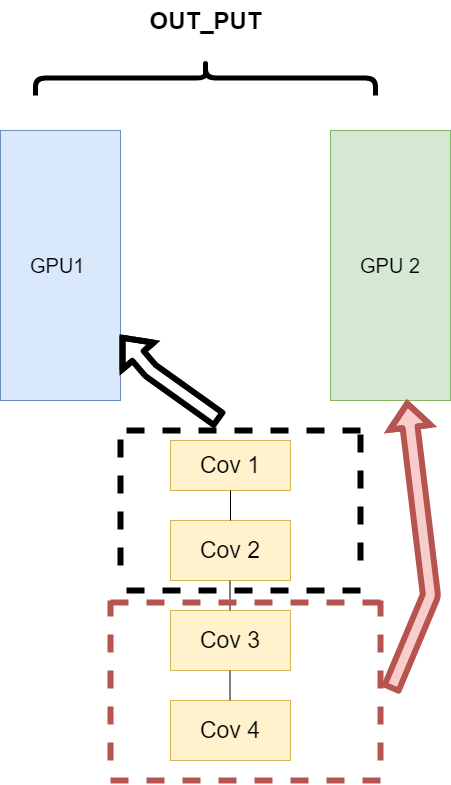
The problem encountered here is that when different model components are on different GPUs, the transmission between GPUs is very important, which is a test for the communication between GPUs. However, GPU communication is difficult to achieve in this intensive task. All this way slowly faded out of sight,

• The tasks of the same layer are distributed to different data (layer wise partitioning)

The second way is to split the model of the same layer and let different GPU s train some tasks of the model of the same layer. Its architecture is as follows:

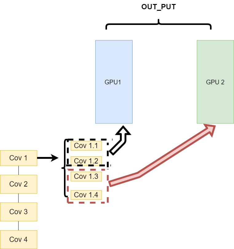
This can ensure the transmission between different components, but when we need a lot of training and the synchronization task is heavier, the same problem as the first method will occur.

• Different data are distributed to different devices to perform the same task (Data parallelism)

The third method is a little different. Its logic is that I will not split the model. When I train, the model is an entire model. But I split the input data. The so-called split data means that after the same model trains part of the data in different GPU s, and then calculates part of the data respectively, it only needs to summarize the output data and then back transmit it. Its architecture is as follows:

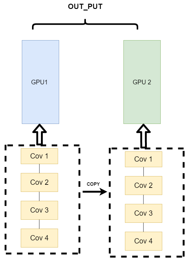
This method can solve the communication problems encountered in the previous mode.

PS: now the mainstream method is Data parallelism

Supplement: feel the concept of tensor through stock data.

In quantitative finance, we use stock data to illustrate the tensors of different dimensions.

Stage 1: a closing price

Steven checked the closing price of Ping An Bank (00000 1.xshe) on January 3, 2019 and found that it was 9.28. He silently saved this single number in X0.

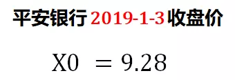
X0 is also called scalar, or more strictly, 0d tensor.

Phase 2: add time dimension

There are too few stock prices in a single day. At least calculate some statistics such as mean and standard deviation.

Steven expanded the data from one day to one year, downloaded the historical closing price of Ping An Bank for the past year from January 3, 2019, and saved it in X1.

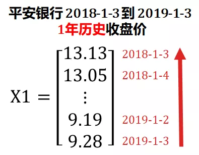
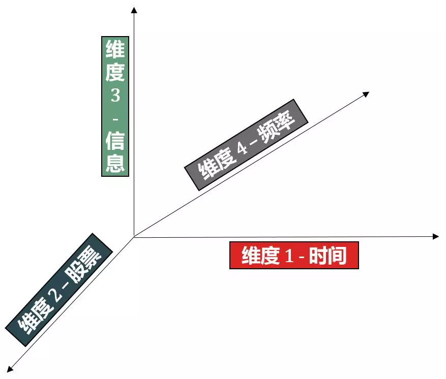
X1 adds the time dimension (red arrow) on the basis of X0, which is extended from scalar to vector, also known as 1D tensor.

Stage 3: add stock dimension

There are too few single stocks. The dispersion principle tells us that we need to invest in two stocks with negative correlation coefficient.

Steven added Maotai stock (600519.XSHG), downloaded the historical closing prices of Ping An Bank and Maotai in the past year from January 3, 2019, and deposited them in X2.

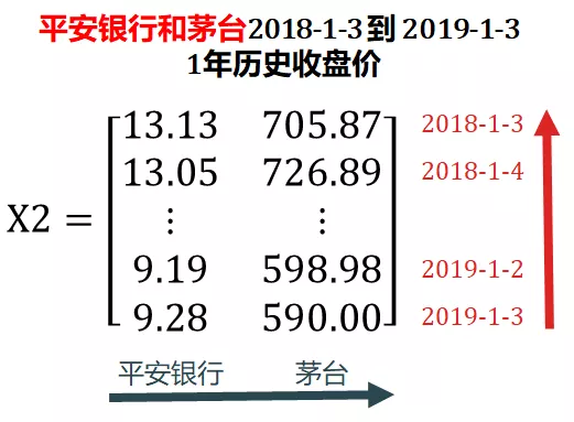
X2 adds a cross-sectional dimension (blue arrow) on the basis of X1, which is extended from vector to matrix, also known as 2D tensor.

Stage 4: add information dimension

The closing price is not enough information. In the trend tracking model, price and trading volume are very important factors in the stock trend.

Steven increased the trading volume, downloaded the historical closing prices and trading volume of Ping An Bank and Maotai in the past year from January 3, 2019, and deposited them in X3.

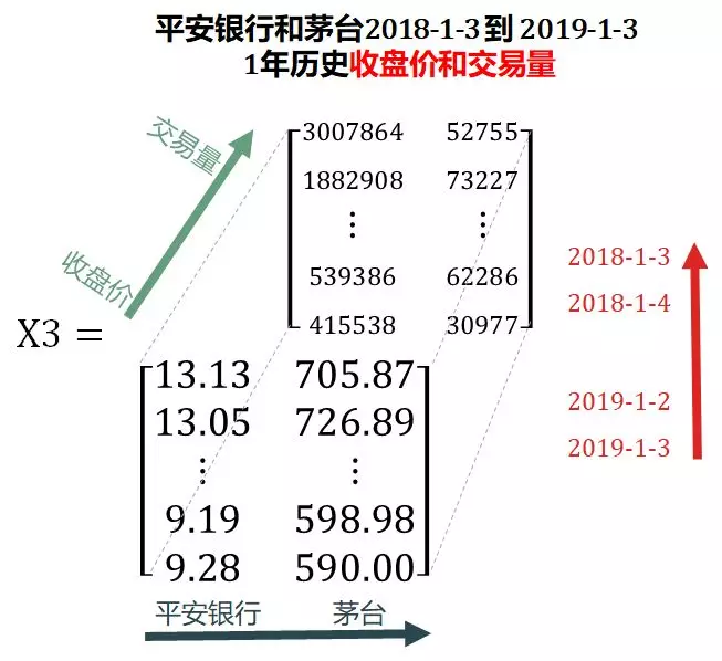
X3 adds an information dimension (green arrow) on the basis of X2, which is extended from the matrix to a three-dimensional tensor (3D tensor).

Phase 5: add frequency dimension

There is too little closing information. What if you want to trade within the day?

Steven added the tick data, downloaded the historical tick prices and transaction volumes of Ping An Bank and Maotai in the past year from January 3, 2019, and saved them in X4.

There are some differences in the definition of tick data between foreign and domestic countries:

• Abroad: any form obtained by changing the order book due to any order.
• Domestic: information sampled according to a certain slice time (500 milliseconds, 3 seconds, 6 seconds, etc.) for the entrusted account book.

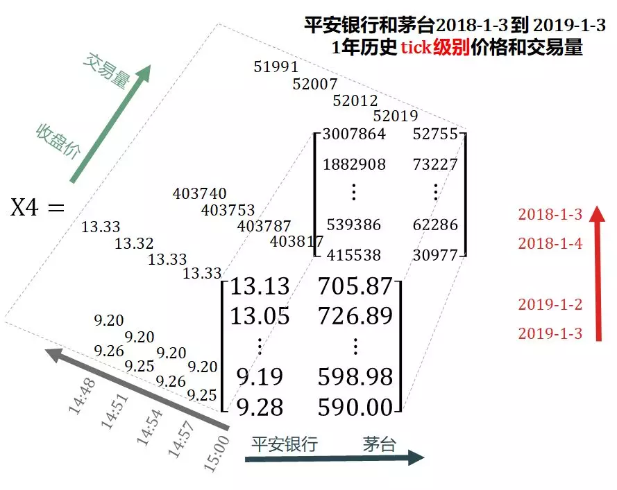
X4 adds the frequency dimension (gray arrow) on the basis of X3, which is expanded from 3D tensor to 4D tensor.