We introduced the distribution hypothesis before, mainly through the context to construct a co-occurrence matrix, cosine similarity, Jaccard similarity and point mutual information can be used to measure the similarity or relevance of words based on the co-occurrence matrix. In order to avoid the statistical unreliability of low-frequency technology, the co-occurrence matrix must be singular decomposed to obtain a more robust low-order representation of the matrix, and then the words are expressed and calculated on the decomposed low-order matrix.

        Distributed representation maps each word to a continuous vector in a low dimensional space. Each dimension has an ambiguous meaning, and the meaning of a word is determined by its vector representation and its spatial relationship with other words.

Word2Vec

        Word vector has become an important part of natural language processing method based on neural network. In the representation method of word vector, each word is marked as a dense space in a low dimensional vector space (generally 100 ~ 1000 dimensions), so that the spatial representation of synonyms is also similar.

        Word2Vec algorithm includes two models CBOW and skip gram for training word vector. The idea of the former is to use multiple words in the context to predict a word, while the idea of the latter is to use each word to predict the context independently. The two are similar

        CBOW model first adds the vectors of all words in the context, then directly calculates the inner product with the vector of the output word, and then normalizes it to the probability distribution. The parameters of the model are composed of two word vector matrices - word output vector matrix and word input vector matrix, which are still optimized by maximum likelihood estimation criterion. This method is more suitable for large-scale data and large word list than feedforward neural network.

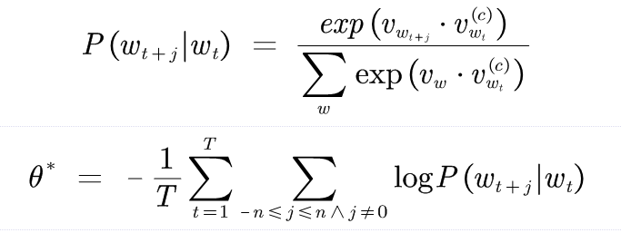
        Compared with the former, skip gram model has stronger independence assumption, that is, each word of the context can also be predicted independently. The model is expressed as follows:

          amongexpressWord vector,DenotationContext word vector.

        Compared with the language model, their optimization goals are the same, but their ultimate goals are different. Language model uses parametric model to estimate conditional probability and predict the next word; Word vector model obtains word vector matrix through conditional probability.

         Although the model is simpler and more efficient, its prediction ability is also much worse. Here are two methods to optimize the calculation cost.

1. Word vector model training Optimization: negative sampling

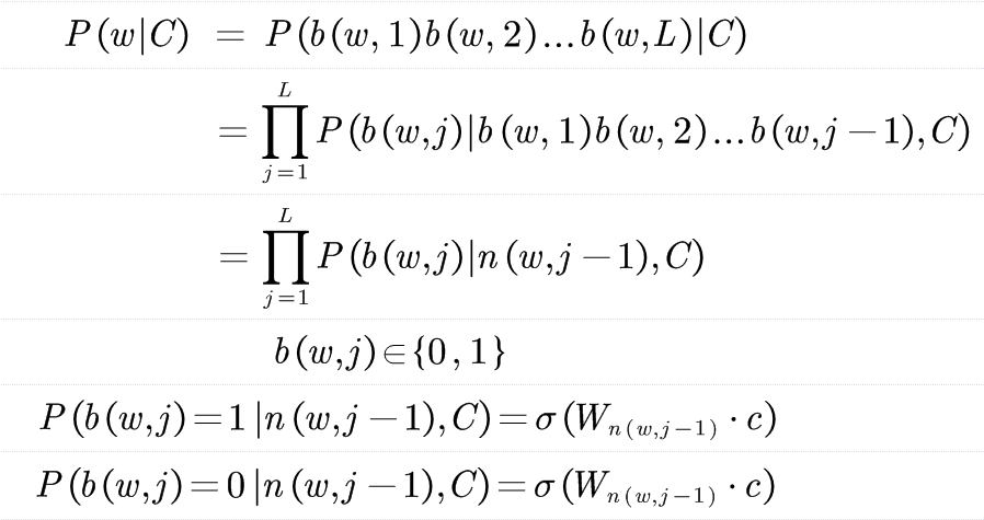
        The negative sampling method transforms the estimation problem of conditional probability into a binary classification problem. If the word w and context c match correctly, B=1, otherwise B=0. The model is as follows:

By using sigmoid function instead of softmax, the calculation of normalization factor is avoided.

2. Word vector model training Optimization: hierarchical softmax

        The main idea is to convert the calculation of normalization factor in softmax into a series of binary classification problems. Firstly, all words in the thesaurus are represented on a binary tree, and each word appears on the leaf node of the tree, corresponding to a unique binary code. In order to optimize the overall cost, Huffman coding can be used.

 

The skip gram code with comments is attached below:

        

# code by Tae Hwan Jung @graykode
import numpy as np
import torch
import torch.nn as nn
import torch.optim as optim
import matplotlib.pyplot as plt

def random_batch():
    random_inputs = []
    random_labels = []
    random_index = np.random.choice(range(len(skip_grams)), batch_size, replace=False)#Randomly select the prediction key pair and predict two at a time
    
    for i in random_index:
        random_inputs.append(np.eye(voc_size)[skip_grams[i][0]])  # target 
        random_labels.append(skip_grams[i][1])  # context word

    return random_inputs, random_labels

# Model
class Word2Vec(nn.Module):
    def __init__(self):
        super(Word2Vec, self).__init__()
        # W and WT is not Traspose relationship
        self.W = nn.Linear(voc_size, embedding_size, bias=False) # voc_ size > embedding_ Size weight maps the unique heat representation value to a point on a two-dimensional plane
        self.WT = nn.Linear(embedding_size, voc_size, bias=False) # embedding_ size > voc_ Size weight then maps the two-dimensional plane points to a vocabulary size vector as the prediction value

    def forward(self, X):
        # X : [batch_size, voc_size]
        hidden_layer = self.W(X) # hidden_layer : [batch_size, embedding_size]
        output_layer = self.WT(hidden_layer) # output_layer : [batch_size, voc_size]
        return output_layer

if __name__ == '__main__':
    batch_size = 2 # mini-batch size
    embedding_size = 2 # embedding size

    sentences = ["apple banana fruit", "banana orange fruit", "orange banana fruit",
                 "dog cat animal", "cat monkey animal", "monkey dog animal"]

    word_sequence = " ".join(sentences).split()
    word_list = " ".join(sentences).split()
    word_list = list(set(word_list))
    word_dict = {w: i for i, w in enumerate(word_list)}
    voc_size = len(word_list)

    # Make skip gram of one size window
    skip_grams = []
    for i in range(1, len(word_sequence) - 1):
        target = word_dict[word_sequence[i]]#Construct key value pairs, select inter words as prediction targets, and words on both sides can be used as context independently
        context = [word_dict[word_sequence[i - 1]], word_dict[word_sequence[i + 1]]]
        for w in context:
            skip_grams.append([target, w])

    model = Word2Vec()

    criterion = nn.CrossEntropyLoss()
    optimizer = optim.Adam(model.parameters(), lr=0.001)

    # Training
    for epoch in range(5000):
        input_batch, target_batch = random_batch()
        input_batch = torch.Tensor(input_batch)
        target_batch = torch.LongTensor(target_batch)#torch.Tensor defaults to torch.FloatTensor, which is 32-bit floating-point data, and torch.LongTensor is 64 bit integer
        
        optimizer.zero_grad()
        output = model(input_batch)
        
        # output : [batch_size, voc_size], target_batch : [batch_size] (LongTensor, not one-hot)
        loss = criterion(output, target_batch)
        if (epoch + 1) % 1000 == 0:
            print('Epoch:', '%04d' % (epoch + 1), 'cost =', '{:.6f}'.format(loss))#Because it is random, there is no intuitive loss drop

        loss.backward()
        optimizer.step()

    for i, label in enumerate(word_list):
        W, WT = model.parameters()
        x, y = W[0][i].item(), W[1][i].item()
        plt.scatter(x, y)#The hidden layer is mapped to a two-dimensional plane for printing, which makes it more intuitive to see that similar words are closer
        plt.annotate(label, xy=(x, y), xytext=(5, 2), textcoords='offset points', ha='right', va='bottom')
    plt.show()

 

  The static word vector can reflect the word vector satisfying a certain transitive relationship (for example, the relationship between brother, sister and grandchildren is similar, only gender difference), which depends on the simplicity of its operation.

But it also brings disadvantages. Due to the lack of context, a word still has the same vector in different contexts despite its different semantics. In addition, there are also problems in the processing of antonyms. The words that are antonyms replace the discourse meaning in the sentence is still smooth, which leads to the possible close distance between the two word vectors. This leads to our current contextual representation model.