1 background knowledge
reference resources:
Heterogeneous Treatment effect aims to quantify the differential impact of the experiment on different populations, and then carry out the differential experiment through population orientation / numerical strategy, or adjust the experiment. Double Machine Learning takes Treatment as a feature and calculates the difference effect of the experiment by estimating the impact of the feature on the target.
Machine Learning is good at giving accurate predictions, while economics pays more attention to the unbiased estimation of the impact of characteristics on objectives. DML combines the method of economics with Machine Learning, and gives an unbiased estimation of the impact of features on the target with an arbitrary ML model under the framework of economics. There is a summary from the boss:

HTE problems can be simply abstracted with the following notation
- Y is the core index of experimental influence
- T is a treatment, usually a 0 / 1 variable, which represents whether the sample enters the experimental group or the control group. For random AB experiment t ⊥ X
- X is a Confounder, which can be simply understood as user features that have not been intervened by experiments, usually high-dimensional vectors
- The final estimate of DML is θ (x) That is, the experiment has different effects on the core indicators of different users

The most direct method is to use X and T to model Y and estimate it directly θ (x).
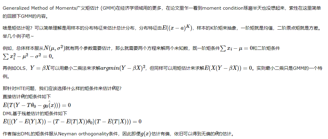
But this estimate θ (x) It is often biased. The deviation comes partly from the over fitting of the sample and partly from the deviation of g(X) estimation. It is assumed that θ If 0 is the true value of the parameter, the deviation is as follows:

2 DML Dynamic Double Machine Learning
[causal inference / uplift modeling] Double Machine Learning(DML)
2.1 DML training process
reference resources: AB experimental population oriented HTE model 4 - Double Machine Learning
Training process:
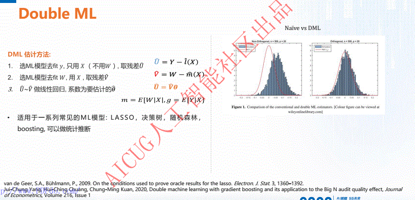
Step 1. Fitting Y and T with any ML model to obtain the residuals Y, t

It is more common to estimate E(Y|x) using lasso / RF
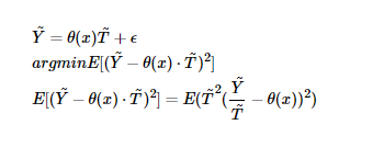
Step 2. Fit y and T with any ML model θ
θ (10) The fitting can be parametric model or nonparametric model, and the parametric model can be fitted directly. The nonparametric model only accepts input and output, so the following transformation is required. The model Target becomes Y/T and the sample weight is T^2
Step 3. Cross fitting
This cross fitting step is very important. A very important step for DML to ensure unbiased estimation is cross fitting, which is used to reduce the estimation deviation caused by overfitting. First divide the total sample into two parts: sample 1 and sample 2.
First, sample 1 is used to estimate the residual, and sample 2 is used to estimate the residual θ 1. Use sample 2 to estimate the residual, and sample 1 to estimate θ 2. Take the average to get the final estimate. Of course, K-Fold can be further used to increase the robustness of the estimation.

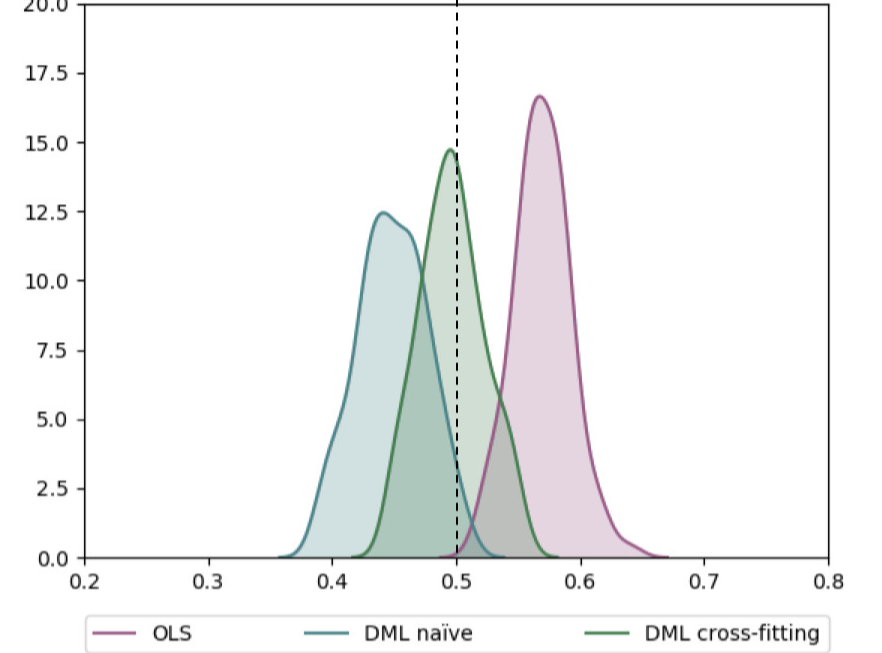
Jonas compares the estimated effects of not using DML, using DML but not cross fitting and using cross fitting in his blog as follows:
2.2 unbiased estimation of HTL
Intuitively, friends familiar with regression here can know that linear regression is the best projection of fitting Y in feature space X (i.e. minimizing the error), so the residual is vertical to sample space X, which eliminates the correlation of (independent) x to the greatest extent! As shown in the figure below.

As for the orthogonalization of residuals, the mathematical principle of unbiased causal effect can be obtained: https://zhuanlan.zhihu.com/p/41993542
Causal inference - Principles and methods (in-depth good article)
2.3 estimating ATE using DML
As for the example of causal inference, we only care about the impact of Treatment T on outcome Y. therefore, we can first use X regression t to obtain a residual of T (actual T - predicted T), then use X regression y to obtain a residual of Y (actual Y - predicted y), and finally use the residual of t to regress the residual of Y, and the estimated parameter is the ATE we want.
( Y − ( Y ∼ X ) ) ∼ ( T − ( T ∼ X ) ) (Y - (Y \sim X)) \sim (T - (T \sim X)) (Y−(Y∼X))∼(T−(T∼X))
Y i − E [ Y i ∣ X i ] = τ ⋅ ( T i − E [ T i ∣ X i ] ) + ϵ Y_i - E[Y_i | X_i] = \tau \cdot (T_i - E[T_i | X_i]) + \epsilon Yi−E[Yi∣Xi]=τ⋅(Ti−E[Ti∣Xi])+ϵ
Therefore, the specific DML method comes out. Its core idea is to use the machine learning algorithm to predict T and Y based on X, and then use the residual of t to regress the residual of Y:
Y i − M ^ y ( X i ) = τ ⋅ ( T i − M ^ t ( X i ) ) + ϵ Y_i - \hat{M}_y(X_i) = \tau \cdot (T_i - \hat{M}_t(X_i)) + \epsilon Yi−M^y(Xi)=τ⋅(Ti−M^t(Xi))+ϵ
Among them, M ^ y ( X i ) \hat{M}_y(X_i) M^y (Xi) modeling E [ Y ∣ X ] E[Y|X] E[Y∣X] , M ^ t ( X i ) \hat{M}_t(X_i) M^t (Xi) modeling E [ T ∣ X ] E[T|X] E[T∣X].
So the question is, why can DML be biased?
The key is M ^ t ( X i ) \hat{M}_t(X_i) M^t (Xi), which depolarizes the Treatment. The residual of t can be regarded as the remaining amount after removing the effect of X on T from T. at this time, the residual of T is independent of X.
and M ^ y ( X i ) \hat{M}_y(X_i) The function of M^y (Xi) is to remove the variance of Y, that is, the variance of Y caused by X is removed from y.
Finally, we model lr the residuals to get ATE.
2.4 estimating CATE using DML
Similarly, we first use ML to obtain the residuals of T and Y based on X, and then use lr to fit the residuals. The difference is that this time we add the interaction terms of X and T, that is
Y i − M y ( X i ) = τ ( X i ) ⋅ ( T i − M t ( X i ) ) + ϵ i Y_i - {M}_y(X_i) = \tau(X_i) \cdot (T_i - {M}_t(X_i)) + \epsilon_i Yi−My(Xi)=τ(Xi)⋅(Ti−Mt(Xi))+ϵi
Y i ~ = α + β 1 T i ~ + β 2 X i T i ~ + ϵ i \tilde{Y_i} = \alpha + \beta_1 \tilde{T_i} + \pmb{\beta}_2 \pmb{X_i} \tilde{T_i} + \epsilon_i Yi~=α+β1Ti~+βββ2XiXiXiTi~+ϵi
Then we can calculate the value of CATE:
μ ^ ( ∂ S a l e s i , X i ) = M ( P r i c e = 1 , X i ) − M ( P r i c e = 0 , X i ) \hat{\mu}(\partial Sales_i, X_i) = M(Price=1, X_i) - M(Price=0, X_i) μ^(∂Salesi,Xi)=M(Price=1,Xi)−M(Price=0,Xi)
Where, M is the last lr model.
2.5 Y of direct prediction counterfactual
When dealing with nonlinear cat, another scheme is that we will no longer try to estimate the linear approximation of cat. Instead, we will make counterfactual predictions.
(this scheme is also widely used in practice, but there is no strict theoretical proof!)
The process is divided into two steps:
The first step is still to estimate the residuals of T and Y:
Y ~ i = τ ( X i ) T ~ i + e i \tilde{Y}_i = \tau(X_i) \tilde{T}_i + e_i Y~i=τ(Xi)T~i+ei
Step 2: Based on the residuals of X and T, use S-learner to predict the residuals of Y:
Y ~ i = τ ( X i , T ~ i ) + e i \tilde{Y}_i = \tau(X_i, \tilde{T}_i) + e_i Y~i=τ(Xi,T~i)+ei
Finally in M ^ y ( X i ) \hat{M}_y(X_i) M^y (Xi) predicted Y ^ \hat{Y} Y ^ plus Y ~ i \tilde{Y}_i Y~i, that is, the final y value is obtained.
3. Relevant cases
3.1 A case of price elasticity realized by DML
come from: Data analysis (29): price demand elasticity and causal inference
3.1.1 price demand elasticity
The economics course talks about price demand elasticity, which describes the elasticity of demand quantity with the change of commodity price. Generally, price does not directly affect demand, but is mediated by intermediate variables related to user decision-making. Assuming Q is the quantity demanded by a commodity and P is the price of the commodity, the price elasticity of demand is,

From the above formula, we can simply know that a price change of 1 yuan will lead to greater demand change than a price change of 100 yuan. For example, 100 units of products can be sold every day at the price of 5 yuan. If the price demand elasticity is - 3, the supplier will increase the price by 5% (dp /P, from 5 yuan - > 5.25 yuan), and the demand will decrease by 15% (dQ/Q, from 100 - > 85). Then the income will decrease by 1005-5.2585 = 53.75.
If the unit price decreases by 5%, the income will increase by 46.25. If the supplier knows the price elasticity of the product, it does not need to test repeatedly to know whether the price should be increased or reduced in order to increase revenue.
3.1.2 DML (Double Machine Learning) solution process
The best way, of course, is to directly conduct A/B experiments to test the response of different prices to users' needs, but exogenous factors such as price will directly damage the user experience by showing different prices to different users at the same stage of the same product. Therefore, causal inference is carried out from the observed historical data, but how to control the confounding factors (seasonality, product quality, etc.) is the challenge of causal inference.
Here, DML (Double Machine Learning) method is used for causal inference, which mainly solves two problems:
- First, the important control variables are selected by regularization;
- Second, compared with the traditional linear regression model, nonparametric inference can solve the nonlinear problem.
DML first applies the machine learning algorithm to fit the result variable Y and the processing variable T through the characteristic variables X and W respectively, and then uses the residual of the processing variable to fit the residual of the result variable through the linear model.
The goal is to estimate that the Y function here is the sum of the causal effect of T and the synergistic effect of X and W.
Divide the data into two parts,
- Part of the samples select random forest model and use mixed variables to predict and process variables (price P) to obtain E[P|X];
- For other samples, the random forest model can also be selected, and the mixed variables are used to predict the result variable (demand Q) to obtain E[Q|X].
Calculate the residuals to obtain the price P and demand Q not affected by hybrid variables, that is:

As for the orthogonalization of residuals, the mathematical principle of unbiased causal effect can be obtained: https://zhuanlan.zhihu.com/p/41993542
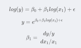
Therefore, the elastic coefficient can be obtained by log log regression of P and Q directly:

About why log log regression can be used to solve the elastic coefficient:
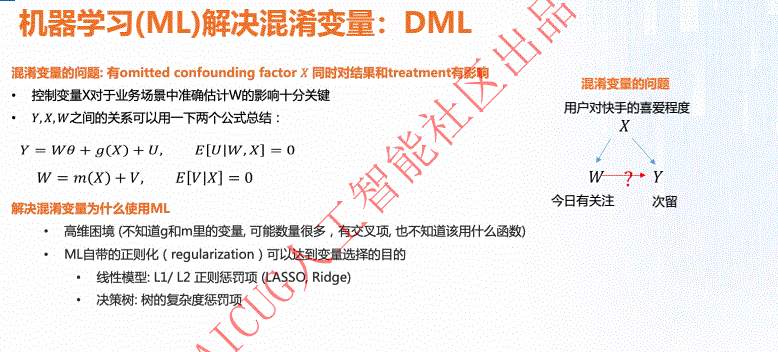
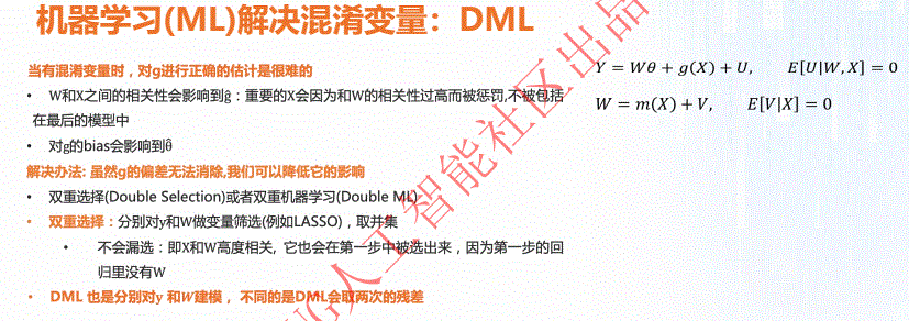
3.2 application of causal analysis tools in Kwai Fu: DML
Article source address: Application of causal analysis tools in Kwai Fu
Kwai: what I think is more interesting is that they give an example: whether the missing variables can be quantified.
- If quantifiable, suitable for DML
For specific PPT, see:

4. Econml's notebook case
4.1 introduction to other theories
reference resources: Journal: causal reasoning
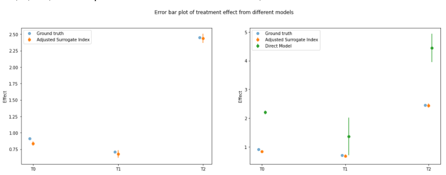
4.1.1 surrogate indexes
Try to use a short-term or easily available intermediate index to replace the long-term or difficult to obtain endpoint index.
Inhibition of arrhythmia can reduce the possibility of cardiac arrest, and [inhibition of arrhythmia] has been used as an alternative index to evaluate [drugs for the treatment of sudden death].
There are many paradoxes caused by confounding factors:
- Yule Simpson paradox: smoking is harmful to men and women respectively, but smoking is beneficial to human beings
- Paradox of surrogate index: arrhythmia is regarded as a surrogate index of sudden death in clinical trials. However, some drugs that can effectively correct arrhythmias were later found not only to reduce sudden death, but also to cause tens of thousands of premature deaths
4.1.2 estimation of dynamic causal effects
https://www.jianshu.com/p/871fbf457a6d
In this framework, a single object plays two roles: processing group and control group at different time points.
When X_t when strictly exogenous, there are two optional dynamic causal effect estimators:
- The first method involves autoregressive distributed lag model (ADL)
- The second method uses the generalized least squares (GLS)
4.2 Double Machine Learning Notebook
Reference official: Double Machine Learning Notebook
There are many small cases in this case:
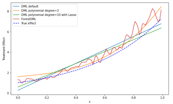
- Example Usage with Single Continuous Treatment Synthetic Data and Model Selection
- Example Usage with Single Binary Treatment Synthetic Data and Confidence Intervals
- Example Usage with Multiple Continuous Treatment Synthetic Data
- Example Usage with Single Continuous Treatment Observational Data
- Example Usage with Multiple Continuous Treatment, Multiple Outcome Observational Data
It includes: t of continuous value, t of secondary classification 01, multiple T and multiple Y
# T of continuous values
array([ 0.41083324,  0.57893171,  1.08130798, ..., -0.43799495,
        1.61941775,  1.64209826])

# T of class II 01
array([0, 0, 0, 0, 1, 1, 0, 1, 1, 1, 0, 0, 0, 0, 1, 0, 1, 0, 1, 0, 0, 0])

# Multi-T
array([[1.35325451, 1.15373159, 0.46373402],
       [1.35325451, 1.15373159, 0.98954119],
       [1.35325451, 0.87129337, 0.73716407],
       ...,
       [1.13462273, 1.03673688, 0.46373402],
       [1.0260416 , 0.95165788, 0.39877612],
       [1.05779029, 0.78390154, 0.55961579]])

# Multi-Y
array([[ 9.01869549,  8.40737833,  9.26482856],
       [ 8.72323127,  8.44934252,  8.98719682],
       [ 8.25322765,  9.91145572,  8.83171192],
       ...,
       [ 9.93653541,  9.51546936,  9.50599061],
       [10.85591733,  9.31793838, 10.9273763 ],
       [10.23652533, 11.20553036,  8.85936345]])
Methods include:
- LinearDML: default
- SparseLinearDML: Polynomial Features for Heterogeneity
- DML: Polynomial Features with regularization
- CausalForestDML: Non-Parametric Heterogeneity with Causal Forest
Including data generation:
import econml
## Ignore warnings
import warnings
warnings.filterwarnings("ignore")

# Main imports
from econml.dml import DML, LinearDML, SparseLinearDML, CausalForestDML

# Helper imports
import numpy as np
from itertools import product
from sklearn.linear_model import (Lasso, LassoCV, LogisticRegression,
                                  LogisticRegressionCV,LinearRegression,
                                  MultiTaskElasticNet,MultiTaskElasticNetCV)
from sklearn.ensemble import RandomForestRegressor,RandomForestClassifier
from sklearn.preprocessing import PolynomialFeatures
import matplotlib.pyplot as plt
import matplotlib
from sklearn.model_selection import train_test_split

%matplotlib inline
# Treatment effect function
def exp_te(x):
    return np.exp(2*x[0])

# DGP constants
np.random.seed(123)
n = 2000
n_w = 30
support_size = 5
n_x = 1
# Outcome support
support_Y = np.random.choice(np.arange(n_w), size=support_size, replace=False)
coefs_Y = np.random.uniform(0, 1, size=support_size)
epsilon_sample = lambda n: np.random.uniform(-1, 1, size=n)
# Treatment support
support_T = support_Y
coefs_T = np.random.uniform(0, 1, size=support_size)
eta_sample = lambda n: np.random.uniform(-1, 1, size=n)

# Generate controls, covariates, treatments and outcomes
W = np.random.normal(0, 1, size=(n, n_w))
X = np.random.uniform(0, 1, size=(n, n_x))
# Heterogeneous treatment effects
TE = np.array([exp_te(x_i) for x_i in X])
T = np.dot(W[:, support_T], coefs_T) + eta_sample(n)
Y = TE * T + np.dot(W[:, support_Y], coefs_Y) + epsilon_sample(n)

Y_train, Y_val, T_train, T_val, X_train, X_val, W_train, W_val = train_test_split(Y, T, X, W, test_size=.2)
# Generate test data
X_test = np.array(list(product(np.arange(0, 1, 0.01), repeat=n_x)))
Model:
# Model
est = LinearDML(model_y=RandomForestRegressor(),
                model_t=RandomForestRegressor(),
                random_state=123)
est.fit(Y_train, T_train, X=X_train, W=W_train)
te_pred = est.effect(X_test)
# Model
est1 = SparseLinearDML(model_y=RandomForestRegressor(),
                       model_t=RandomForestRegressor(),
                       featurizer=PolynomialFeatures(degree=3),
                       random_state=123)
est1.fit(Y_train, T_train, X=X_train, W=W_train)
te_pred1 = est1.effect(X_test)

# Model
est2 = DML(model_y=RandomForestRegressor(),
           model_t=RandomForestRegressor(),
           model_final=Lasso(alpha=0.1, fit_intercept=False),
           featurizer=PolynomialFeatures(degree=10),
           random_state=123)
est2.fit(Y_train, T_train, X=X_train, W=W_train)
te_pred2 = est2.effect(X_test)
# Model
est3 = CausalForestDML(model_y=RandomForestRegressor(),
                       model_t=RandomForestRegressor(),
                       criterion='mse', n_estimators=1000,
                       min_impurity_decrease=0.001,
                       random_state=123)
est3.tune(Y_train, T_train, X=X_train, W=W_train)
est3.fit(Y_train, T_train, X=X_train, W=W_train)
te_pred3 = est3.effect(X_test)

# Drawing
plt.figure(figsize=(10,6))
plt.plot(X_test, te_pred, label='DML default')
plt.plot(X_test, te_pred1, label='DML polynomial degree=3')
plt.plot(X_test, te_pred2, label='DML polynomial degree=10 with Lasso')
plt.plot(X_test, te_pred3, label='ForestDML')
expected_te = np.array([exp_te(x_i) for x_i in X_test])
plt.plot(X_test, expected_te, 'b--', label='True effect')
plt.ylabel('Treatment Effect')
plt.xlabel('x')
plt.legend()
plt.show()
The following includes model selection:
score={}
score["DML default"] = est.score(Y_val, T_val, X_val, W_val)
score["DML polynomial degree=3"] = est1.score(Y_val, T_val, X_val, W_val)
score["DML polynomial degree=10 with Lasso"] = est2.score(Y_val, T_val, X_val, W_val)
score["ForestDML"] = est3.score(Y_val, T_val, X_val, W_val)

mse_te={}
mse_te["DML default"] = ((expected_te - te_pred)**2).mean()
mse_te["DML polynomial degree=3"] = ((expected_te - te_pred1)**2).mean()
mse_te["DML polynomial degree=10 with Lasso"] = ((expected_te - te_pred2)**2).mean()
mse_te["ForestDML"] = ((expected_te - te_pred3)**2).mean()

print("best model selected by MSE of TE: ", min(mse_te, key=lambda x: mse_te.get(x)))
score refers to MSE, the smaller the better
4.3 Dynamic Double Machine Learning Examples
reference resources: Dynamic Double Machine Learning Examples.ipynb
Dynamic DoubleML is an extension of the Double ML approach for treatments assigned sequentially over time periods. This estimator will account for treatments that can have causal effects on future outcomes.
It is equivalent to DML + timing effect, so it is generally required for panel data
Generate data
import econml
# Main imports
from econml.dynamic.dml import DynamicDML
from econml.tests.dgp import DynamicPanelDGP, add_vlines

# Helper imports
import numpy as np
from sklearn.linear_model import Lasso, LassoCV, LogisticRegression, LogisticRegressionCV, MultiTaskLassoCV
import matplotlib.pyplot as plt

%matplotlib inline

# Define DGP parameters
np.random.seed(123)
n_panels = 5000 # number of panels
n_periods = 3 # number of time periods in each panel
n_treatments = 2 # number of treatments in each period
n_x = 100 # number of features + controls
s_x = 10 # number of controls (endogeneous variables)
s_t = 10 # treatment support size

# Generate data
dgp = DynamicPanelDGP(n_periods, n_treatments, n_x).create_instance(
            s_x, random_seed=12345)
Y, T, X, W, groups = dgp.observational_data(n_panels, s_t=s_t, random_seed=12345)
true_effect = dgp.true_effect
You can see the panel data, including three-year data, 5000 samples and two processing T
model training
# Train Estimator
est = DynamicDML(
    model_y=LassoCV(cv=3, max_iter=1000),
    model_t=MultiTaskLassoCV(cv=3, max_iter=1000),
    cv=3)
est.fit(Y, T, X=None, W=W, groups=groups)

# Effect of target policy over baseline policy
# Must specify a treatment for each period
baseline_policy = np.zeros((1, n_periods * n_treatments))
target_policy = np.ones((1, n_periods * n_treatments))
eff = est.effect(T0=baseline_policy, T1=target_policy)
print(f"Effect of target policy over baseline policy: {eff[0]:0.2f}")

# Period treatment effects + interpretation
for i, theta in enumerate(est.intercept_.reshape(-1, n_treatments)):
    print(f"Marginal effect of a treatments in period {i+1} on period {n_periods} outcome: {theta}")

# Period treatment effects with confidence intervals
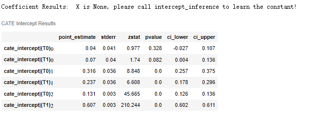
est.summary()

conf_ints = est.intercept__interval(alpha=0.05)
You can know the situation of CATE:
Drawing:
# Some plotting boilerplate code
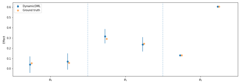
plt.figure(figsize=(15, 5))
plt.errorbar(np.arange(n_periods*n_treatments)-.04, est.intercept_, yerr=(conf_ints[1] - est.intercept_,
                                                    est.intercept_ - conf_ints[0]), fmt='o', label='DynamicDML')
plt.errorbar(np.arange(n_periods*n_treatments), true_effect.flatten(), fmt='o', alpha=.6, label='Ground truth')
for t in np.arange(1, n_periods):
    plt.axvline(x=t * n_treatments - .5, linestyle='--', alpha=.4)
plt.xticks([t * n_treatments - .5 + n_treatments/2 for t in range(n_periods)],
           ["$\\theta_{}$".format(t) for t in range(n_periods)])
plt.gca().set_xlim([-.5, n_periods*n_treatments - .5])
plt.ylabel("Effect")
plt.legend()
plt.show()
4.4 Long-Term Return-on-Investment at Microsoft via Short-Term Proxies
Case Study - Long-Term Return-on-Investment at Microsoft via Short-Term Proxies.ipynb
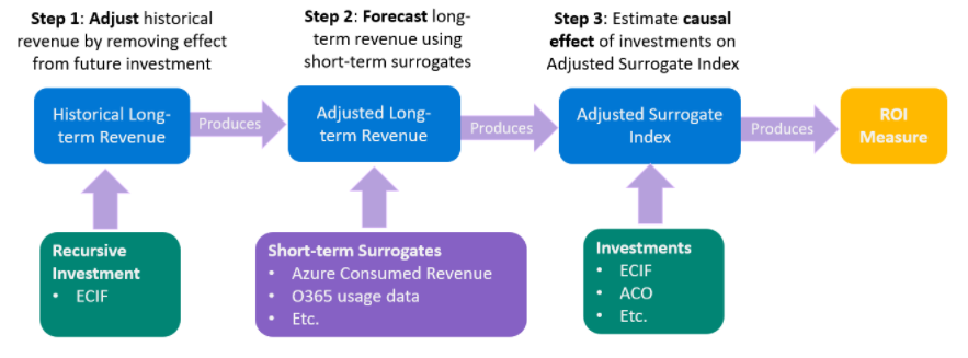
Here is a very difficult case about dynamic DML. When I read it, I find it very difficult to understand. The substitute indicators in [4.1] are also involved here.
According to the author's understanding, the following is a summary to generate data:
# imports
from econml.data.dynamic_panel_dgp import SemiSynthetic
from sklearn.linear_model import LassoCV, MultiTaskLassoCV
import numpy as np
import matplotlib.pyplot as plt

# generate historical dataset (training purpose)
np.random.seed(43)
dgp = SemiSynthetic()
dgp.create_instance()
n_periods = 4    # Y contains several periods, and the default is 4 periods
n_units = 5000   # sample size
n_treatments = dgp.n_treatments  # 3 - Multi intervention
random_seed = 43
thetas = np.random.uniform(0, 2, size=(dgp.n_proxies, n_treatments))  # Error term

panelX, panelT, panelY, panelGroups, true_effect = dgp.gen_data(
    n_units, n_periods, thetas, random_seed
)
Here are four years (periods) of data, 5k sample size for each period
4.4.1 obtain control Y without processing through DynamicDML
The DynamicDML result is uplift increment, Y real value - DynamicDML increment = Y regular trend
This is a bit like the decomposition of time series, which is divided into: long-term trend, seasonal variation, cyclic fluctuation and irregular fluctuation
EconML's DynamicDML estimator is an extension of Double Machine Learning approach to dynamically estimate the period effect of treatments assigned sequentially over time period. In this scenario, it could help us to adjust the cumulative revenue by subtracting the period effect of all of the investments after the target investment.
# on historical data construct adjusted outcomes
from econml.dynamic.dml import DynamicDML

panelYadj = panelY.copy()

est = DynamicDML(
    model_y=LassoCV(max_iter=2000), model_t=MultiTaskLassoCV(max_iter=2000), cv=2
)
for t in range(1, n_periods):  # for each target period 1...m
    # learn period effect for each period treatment on target period t
    est.fit(
        long(panelY[:, 1 : t + 1]),
        long(panelT[:, 1 : t + 1, :]),  # reshape data to long format
        X=None,
        W=long(panelX[:, 1 : t + 1, :]),
        groups=long(panelGroups[:, 1 : t + 1]),
    )
    # print(f'y's shape {long (panely [:, 1: T + 1]). Shape}, t is {t}, x is {long (panelx [:, 1: T + 1,:]. Shape} ')
    # remove effect of observed treatments
    T1 = wide(panelT[:, 1 : t + 1, :])
    panelYadj[:, t] = panelY[:, t] - est.effect(
        T0=np.zeros_like(T1), T1=T1
    )  # reshape data to wide format
In the process of repairing each phase, the dynamic DML trained with data is also inconsistent;
For example, if the first period has only 5000 samples, take 5000 samples first;
The second period is 5000 samples from the first period + the second period, a total of 10000 samples.
The whole case is very incomprehensible because these data have no practical significance, and the author can only understand it according to,
It is assumed that this data is to predict the impact of bank interest rate hikes, interest rate cuts, new derivatives (T1/T2/T3, all continuous values) and population, economy (X/W) and other factors on the GDP (Y) of 5000 countries in four years
The first elimination operation is to remove the impact of bank interest rate increase, interest rate cut and new derivatives, leaving separate demographic / economic factors, and then solve the Adjusted GDP
4.4.2 short term time series as a substitute index for long-term time series
# A Y ~ X regression model is trained separately for prediction
# train surrogate index on historical dataset
XS = np.hstack(
    [panelX[:, 1], panelYadj[:, :1]]
)  # concatenate controls and surrogates from historical dataset
# There are four periods, the second period of X / Y
# (5000, 71) + (5000, 1) => (5000, 72)

TotalYadj = np.sum(panelYadj, axis=1)  # total revenue from historical dataset
adjusted_proxy_model = LassoCV().fit(
    XS, TotalYadj
)  # train proxy model from historical dataset


# predict new long term revenue
XSnew = np.hstack(
    [panelXnew[:, 1], panelYnew[:, :1]]
)  # concatenate controls and surrogates from new dataset
sindex_adj = adjusted_proxy_model.predict(XSnew)
It's still difficult to understand here, because the explanation of data use is not careful enough (or I don't understand...):
If we want to predict the total Adjusted GDP of these 5000 countries in the next four years
Based on the training model of the results of the previous four years, an assumption made here is to take the first year as the short-term replacement of all four years to predict all GDP in the next four years. Steps:
- LassoCV training: X in year 1 ~ Y in the past 4 years
- Forecast for the next four years: X of this year ~ Y of the next four years
So we get the adjusted estimate Y for the next four years
There should also be [4.4.3 evaluation of policy effect: difference between actual Y and estimated + adjusted Y]
There is a comparison of linear DML estimates of X|W based on adjusted Y and actual Y, but I don't understand this feeling, so I'll write it here for the time being.
