This tutorial creates a small neural network for handwritten character recognition. We use MNIST data sets for training and testing. The training set of this data set contains 60,000 images of handwritten characters from 500 people, and the test set contains 10,000 test images independent of the training set. You can refer to this tutorial. Ipython notebook.

In this section, we use the model assistant of CNN to create the network and initialize the parameters. First import the required dependency libraries.

%matplotlib inline
from matplotlib import pyplot
import numpy as np
import os
import shutil
from caffe2.python import core, cnn, net_drawer, workspace, visualize
# If you want to know more about the initialization process, you can change caffe2_log_level=0 to -1.
core.GlobalInit(['caffe2', '--caffe2_log_level=0'])
caffe2_root = "~/caffe2"
print("Necessities imported!")

Data preparation

We will track the training process data and save it to a local folder. We need to set up a data file and root folder first. In the data folder, place the MNIST data set for training and testing. If there is no data set, you can download it here. MNIST Dataset Then decompress the data set and labels.

./make_mnist_db --channel_first --db leveldb --image_file ~/Downloads/train-images-idx3-ubyte --label_file ~/Downloads/train-labels-idx1-ubyte --output_file ~/caffe2/caffe2/python/tutorials/tutorial_data/mnist/mnist-train-nchw-leveldb

./make_mnist_db --channel_first --db leveldb --image_file ~/Downloads/t10k-images-idx3-ubyte --label_file ~/Downloads/t10k-labels-idx1-ubyte --output_file ~/caffe2/caffe2/python/tutorials/tutorial_data/mnist/mnist-test-nchw-leveldb

This code implements the same functionality as above

# This section converts your image into leveldb
current_folder = os.getcwd()
data_folder = os.path.join(current_folder, 'tutorial_data', 'mnist')
root_folder = os.path.join(current_folder, 'tutorial_files', 'tutorial_mnist')
image_file_train = os.path.join(data_folder, "train-images-idx3-ubyte")
label_file_train = os.path.join(data_folder, "train-labels-idx1-ubyte")
image_file_test = os.path.join(data_folder, "t10k-images-idx3-ubyte")
label_file_test = os.path.join(data_folder, "t10k-labels-idx1-ubyte")

def DownloadDataset(url, path):
    import requests, zipfile, StringIO
    print "Downloading... ", url, " to ", path
    r = requests.get(url, stream=True)
    z = zipfile.ZipFile(StringIO.StringIO(r.content))
    z.extractall(path)
if not os.path.exists(data_folder):
    os.makedirs(data_folder)
if not os.path.exists(label_file_train):
    DownloadDataset("https://s3.amazonaws.com/caffe2/datasets/mnist/mnist.zip", data_folder)

def GenerateDB(image, label, name):
    name = os.path.join(data_folder, name)
    print 'DB name: ', name
    syscall = "/usr/local/binaries/make_mnist_db --channel_first --db leveldb --image_file " + image + " --label_file " + label + " --output_file " + name
    print "Creating database with: ", syscall
    os.system(syscall)

# Generating leveldb
GenerateDB(image_file_train, label_file_train, "mnist-train-nchw-leveldb")
GenerateDB(image_file_test, label_file_test, "mnist-test-nchw-leveldb")

if os.path.exists(root_folder):
    print("Looks like you ran this before, so we need to cleanup those old workspace files...")
    shutil.rmtree(root_folder)

os.makedirs(root_folder)
workspace.ResetWorkspace(root_folder)

print("training data folder:"+data_folder)
print("workspace root folder:"+root_folder)

Model establishment

CNNModelHelper encapsulates many functions, which can initialize parameters and implement real calculations in two networks. The underlying implementation is that CNNModelHelper has two networks, param_init_net and net, which record the initialization network and the main network respectively. In order to modularize, we divide the model into several different parts.

- Data input (AddInput function)
- The main computational part (AddLeNetModel function)
- Training part - Gradient operation, parameter update, etc. (AddTrainingOperators function)
- Record the data section, such as the data needed to show the training process (AddBookkeeping Operators function)

1. AddInput loads data from a DB. We save MNIST as a pixel value, and we compute with floating point numbers, so our data must also be Float type. For numerical stability, we normalize the image data to [0,1] instead of [0,255]. Note that what we do in-place overrides the original data, because we don't need pre-normalized data. The operation of preparing data does not require gradient calculation when propagating backwards. So we use StopGradient to tell the gradient generator, "Don't pass the gradient to me."

   def AddInput(model, batch_size, db, db_type):
    # Load data and labels
    data_uint8, label = model.TensorProtosDBInput(
        [], ["data_uint8", "label"], batch_size=batch_size,
        db=db, db_type=db_type)
    # Convert to float
    data = model.Cast(data_uint8, "data", to=core.DataType.FLOAT)
    #Normalization to [0,1]
    data = model.Scale(data, data, scale=float(1./256))
    # Backward propagation does not require gradients
    data = model.StopGradient(data, data)
    return data, label
   print("Input function created.")

   output

   Input function created.

2. AddLeNetModel outputs softmax.

   def AddLeNetModel(model, data):
    conv1 = model.Conv(data, 'conv1', 1, 20, 5)
    pool1 = model.MaxPool(conv1, 'pool1', kernel=2, stride=2)
    conv2 = model.Conv(pool1, 'conv2', 20, 50, 5)
    pool2 = model.MaxPool(conv2, 'pool2', kernel=2, stride=2)
    fc3 = model.FC(pool2, 'fc3', 50 * 4 * 4, 500)
    fc3 = model.Relu(fc3, fc3)
    pred = model.FC(fc3, 'pred', 500, 10)
    softmax = model.Softmax(pred, 'softmax')
    return softmax
   print("Model function created.")

   Model function created.

3. The AddTrainingOperators function is used to add training operations.
   The AddAccuracy function outputs the accuracy of the model, which we will use in the next function to track the accuracy.

   def AddAccuracy(model, softmax, label):
    accuracy = model.Accuracy([softmax, label], "accuracy")
    return accuracy
   print("Accuracy function created.")

   Accuracy function created.

   First, an op: LabelCrossEntropy is added to calculate the cross-entropy of input and lebel. This operation is done after the software Max is obtained and before loss is calculated. The input is [soft max, label], and the output cross-entropy is expressed by xent.

   xent = model.LabelCrossEntropy([softmax, label], 'xent')

   AveragedLoss takes cross-entropy as input and calculates average loss.

   loss = model.AveragedLoss(xent, "loss")

   In order to record the training process, we use the AddAccuracy function to calculate.

   AddAccuracy(model, softmax, label)

   The next step is crucial: we add all the gradient calculations to the model. The gradient is calculated from loss in front of us.

   model.AddGradientOperators([loss])

   Then enter the iteration.

   ITER = model.Iter("iter")

   The strategy of updating learning rate is LR = base_lr* (t ^ gamma). Note that we are minimizing, so the basic learning rate is negative, so that we can go downhill.

   LR = model.LearningRate(ITER, "LR", base_lr=-0.1, policy="step", stepsize=1, gamma=0.999 ) 
   #ONE is a constant used in the gradient renewal stage. It only needs to be created once and placed in param_init_net.
   ONE = model.param_init_net.ConstantFill([], "ONE", shape=[1], value=1.0)

   Now for each parameter, we do gradient updates. Notice how we get the gradient of each parameter -- CNNModelHelper keeps track of this information. The way to update is simple, simple addition: param = param + param_grad * LR

   for param in model.params:
    param_grad = model.param_to_grad[param]
    model.WeightedSum([param, ONE, param_grad, LR], param)

   We need to check the parameters every once in a while. This can be done through Checkpoint. This operation has a parameter Every to indicate how many iterations this operation is performed once to prevent too frequent checks. Here, we do a check every 20 iterations.

   model.Checkpoint([ITER] + model.params, [],
               db="mnist_lenet_checkpoint_%05d.leveldb",
               db_type="leveldb", every=20)

   Then we get the whole AddTrainingOperators function as follows:

   def AddTrainingOperators(model, softmax, label):
    # Computation of Cross Entropy
    xent = model.LabelCrossEntropy([softmax, label], 'xent')
    # Calculate loss
    loss = model.AveragedLoss(xent, "loss")
    #Accuracy of tracking model
    AddAccuracy(model, softmax, label)
    #Adding gradient operation
    model.AddGradientOperators([loss])
    # gradient descent
    ITER = model.Iter("iter")
    # learning rate
    LR = model.LearningRate(
        ITER, "LR", base_lr=-0.1, policy="step", stepsize=1, gamma=0.999 )
    ONE = model.param_init_net.ConstantFill([], "ONE", shape=[1], value=1.0)
    # Gradient update
    for param in model.params:
        param_grad = model.param_to_grad[param]
        model.WeightedSum([param, ONE, param_grad, LR], param)
    # Check 20 times per iteration
    # you may need to delete tutorial_files/tutorial-mnist to re-run the tutorial
    model.Checkpoint([ITER] + model.params, [],
                   db="mnist_lenet_checkpoint_%05d.leveldb",
                   db_type="leveldb", every=20)
   print("Training function created.")

   Training function created.

4. AddBookkeeping Operators add some recording operations that do not affect the training process. They just collect data and print it out or write it into the log.

   def AddBookkeepingOperators(model):
    # Output the content of the blob. to_file=1 means output to the file. The path to save the file is root_folder/[blob name]
    model.Print('accuracy', [], to_file=1)
    model.Print('loss', [], to_file=1)
    # Summarizes gives some parameters such as mean, variance, maximum and minimum.
    for param in model.params:
        model.Summarize(param, [], to_file=1)
        model.Summarize(model.param_to_grad[param], [], to_file=1)
   print("Bookkeeping function created")

5. Defining network
   Now let's actually create the model. The functions written above will actually be executed. Recall our four steps.

   -data input  
   -main computation
   -training
   -bookkeeping

   Before we read in the data, we need to define our training model. We'll use everything we defined earlier. We will use NCHW storage order on the MINIST dataset.

train_model = cnn.CNNModelHelper(order="NCHW", name="mnist_train")
data, label = AddInput(train_model, batch_size=64,
              db=os.path.join(data_folder, 'mnist-train-nchw-leveldb'), db_type='leveldb')
softmax = AddLeNetModel(train_model, data)
AddTrainingOperators(train_model, softmax, label)
AddBookkeepingOperators(train_model)
# Testing model. We set batch=100 so that 100 iterations can cover 10,000 test images.
# For the test model, we need three parts: data input, LeNetModel, and accuracy.
#Notice that init_params is set to False because we get parameters from the training network.
test_model = cnn.CNNModelHelper(order="NCHW", name="mnist_test", init_params=False)
data, label = AddInput(test_model, batch_size=100,
    db=os.path.join(data_folder, 'mnist-test-nchw-leveldb'), db_type='leveldb')
softmax = AddLeNetModel(test_model, data)
AddAccuracy(test_model, softmax, label)

# Deployment model. We only need the LeNetModel section
deploy_model = cnn.CNNModelHelper(order="NCHW", name="mnist_deploy", init_params=False)
AddLeNetModel(deploy_model, "data")
#You may be curious about what happened to param_init_net of deploy_model, which we did not use in this section.
#Because in the deployment phase, we do not randomly initialize parameters, but load them locally.
print('Created training and deploy models.')

Now let's use the caffe2 visualization tool to see what the Training and Deploy models look like. If the following command fails, it may be because your machine does not install graphviz. You can install it with the following commands:

sudo yum install graphviz #ubuntu user sudo apt-get install graphviz

The graph may look small, and you can see it by right-clicking in a new window.

from IPython import display
graph = net_drawer.GetPydotGraph(train_model.net.Proto().op, "mnist", rankdir="LR")
display.Image(graph.create_png(), width=800)

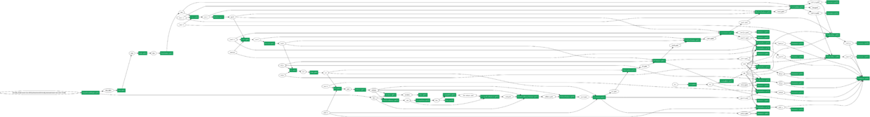
Now the picture above shows everything at the training stage. White nodes are blobs and green rectangular nodes are operators. You may notice large parallel lines like railway tracks. These dependencies point from forward-propagating blobs to backward-propagating operations.
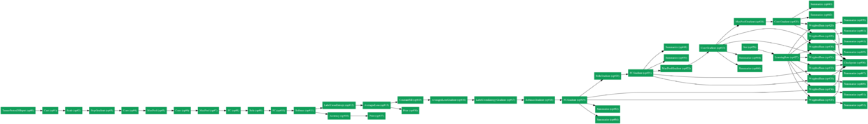
Let's just show the necessary dependencies and operations. If you look carefully, you will find that the left half of the schema propagates forward, the right half of the schema propagates backward, and on the far right is a series of parameter update operations and summarization.

graph = net_drawer.GetPydotGraphMinimal(
    train_model.net.Proto().op, "mnist", rankdir="LR", minimal_dependency=True)
display.Image(graph.create_png(), width=800)

Now we can run the network through Python. Remember, when we run the network, we can always pull out blob data from the network. Here's how to do this.

Let's reiterate that the CNNModelHelper class currently does nothing. What he's doing now is just declaring the network and simply creating protocol buffers. For example, we can show a part of the serialized protobuf of the network.

print(str(train_model.param_init_net.Proto())[:400] + '\n...')

Of course, we can also write protobuf to the local disk, so that it can be easily viewed. You will find that these protobufs are very similar to previous Caffe network definitions.

with open(os.path.join(root_folder, "train_net.pbtxt"), 'w') as fid:
    fid.write(str(train_model.net.Proto()))
with open(os.path.join(root_folder, "train_init_net.pbtxt"), 'w') as fid:
    fid.write(str(train_model.param_init_net.Proto()))
with open(os.path.join(root_folder, "test_net.pbtxt"), 'w') as fid:
    fid.write(str(test_model.net.Proto()))
with open(os.path.join(root_folder, "test_init_net.pbtxt"), 'w') as fid:
    fid.write(str(test_model.param_init_net.Proto()))
with open(os.path.join(root_folder, "deploy_net.pbtxt"), 'w') as fid:
    fid.write(str(deploy_model.net.Proto()))
print("Protocol buffers files have been created in your root folder: "+root_folder)

Now let's get into the training process. We use Python to train. Of course, you can also use the C++ interface to train. This will be discussed in another tutorial.

Training network

First of all, it is necessary to initialize the network

workspace.RunNetOnce(train_model.param_init_net)

Then we create a training network and load it into workspace.

workspace.CreateNet(train_model.net)

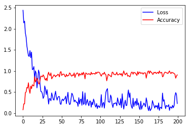
Then set up 200 iterations and save the accuracy and loss into two np matrices.

total_iters = 200
accuracy = np.zeros(total_iters)
loss = np.zeros(total_iters)

After the network and trace accurate loss are configured, we call workspace. RunNet 200 times, and the parameter we need to pass in is train_model.net.Proto().name. For each iteration, we calculate the accuracy and loss.

for i in range(total_iters):
    workspace.RunNet(train_model.net.Proto().name)
    accuracy[i] = workspace.FetchBlob('accuracy')
    loss[i] = workspace.FetchBlob('loss')

Finally, we can draw the result with pyplot.

# Parameter initialization only needs to run once
workspace.RunNetOnce(train_model.param_init_net)
# Create network
workspace.CreateNet(train_model.net)
#Setting the number of iterations and tracking accuracy & loss
total_iters = 200
accuracy = np.zeros(total_iters)
loss = np.zeros(total_iters)
# We iterate 200 times.
for i in range(total_iters):
    workspace.RunNet(train_model.net.Proto().name)
    accuracy[i] = workspace.FetchBlob('accuracy')
    loss[i] = workspace.FetchBlob('loss')
# Iterative completion draws results
pyplot.plot(loss, 'b')
pyplot.plot(accuracy, 'r')
pyplot.legend(('Loss', 'Accuracy'), loc='upper right')

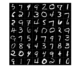
Now we can extract data and make predictions.

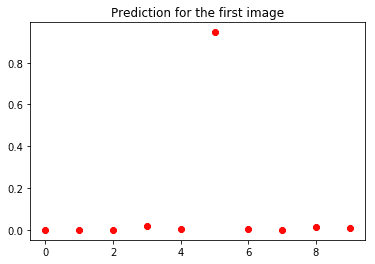
#Data visualization
pyplot.figure()
data = workspace.FetchBlob('data')
_ = visualize.NCHW.ShowMultiple(data)
pyplot.figure()
softmax = workspace.FetchBlob('softmax')
_ = pyplot.plot(softmax[0], 'ro')
pyplot.title('Prediction for the first image')

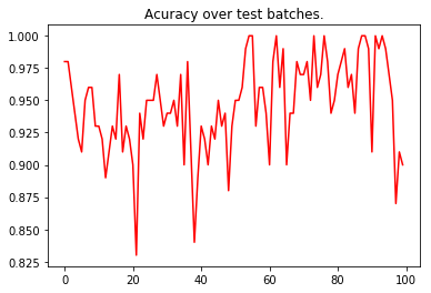
Remember the test net we created? We will run the test net once to test the accuracy. Note that although the parameters of test_model come from train_model, you still need to initialize test_model.param_init_net. This time, we only need to track the accuracy, and only iterate 100 times.

workspace.RunNetOnce(test_model.param_init_net)
workspace.CreateNet(test_model.net)
test_accuracy = np.zeros(100)
for i in range(100):
    workspace.RunNet(test_model.net.Proto().name)
    test_accuracy[i] = workspace.FetchBlob('accuracy')
pyplot.plot(test_accuracy, 'r')
pyplot.title('Acuracy over test batches.')
print('test_accuracy: %f' % test_accuracy.mean())

Translator's Note: The translator here does not quite understand how test_model gets parameters from train_model. There are clear partners who would like to share them in the comments section.

This concludes the MNIST tutorial. I hope this tutorial will show you some features of Caffe2.

For reprinting, please indicate the source: http://www.jianshu.com/c/cf07b31bb5f2