Copyright is owned by Mr. Wu Enda for reference. Koala_Tree'sBlog Some of them are added according to their own practice

Using google translation, part of manual translation

Part 1: Construction of deep neural network:

1 - bag

Let's first import all the packages you need during this allocation.  
- numpy Python is the main software package for scientific computing.
- matplotlib It's a library of graphics drawn with Python.
- dnn_utils provides some necessary functions for this notebook.
- TesCases provides some test cases to evaluate the correctness of functions
- np.random.seed (1) is used to maintain the consistency of all random function calls. It will help us evaluate your work. Please don't change the seeds.

import numpy as np 
import h5py
import matplotlib.pyplot as plt 
from testCases_v3 import *
from dnn_utils_v2 import sigmoid,sigmoid_backward,relu,relu_backward

plt.rcParams["figure.figsize"]=(5.0,4.0)
plt.rcParams["image.interpolation"]="nearset"
plt.rcParams["image.cmap"]="gray"

np.random.seed(1)

2 - Operational summary

To build your neural network, you will implement several "auxiliary functions". These auxiliary functions will be used for the next task to construct a two-layer neural network and an L-layer neural network. Each small assistant function you will implement will provide detailed instructions to guide you through the necessary steps. Following is a summary of this assignment. You will:

• Initialize the parameters of the two-layer network and L-layer neural network.
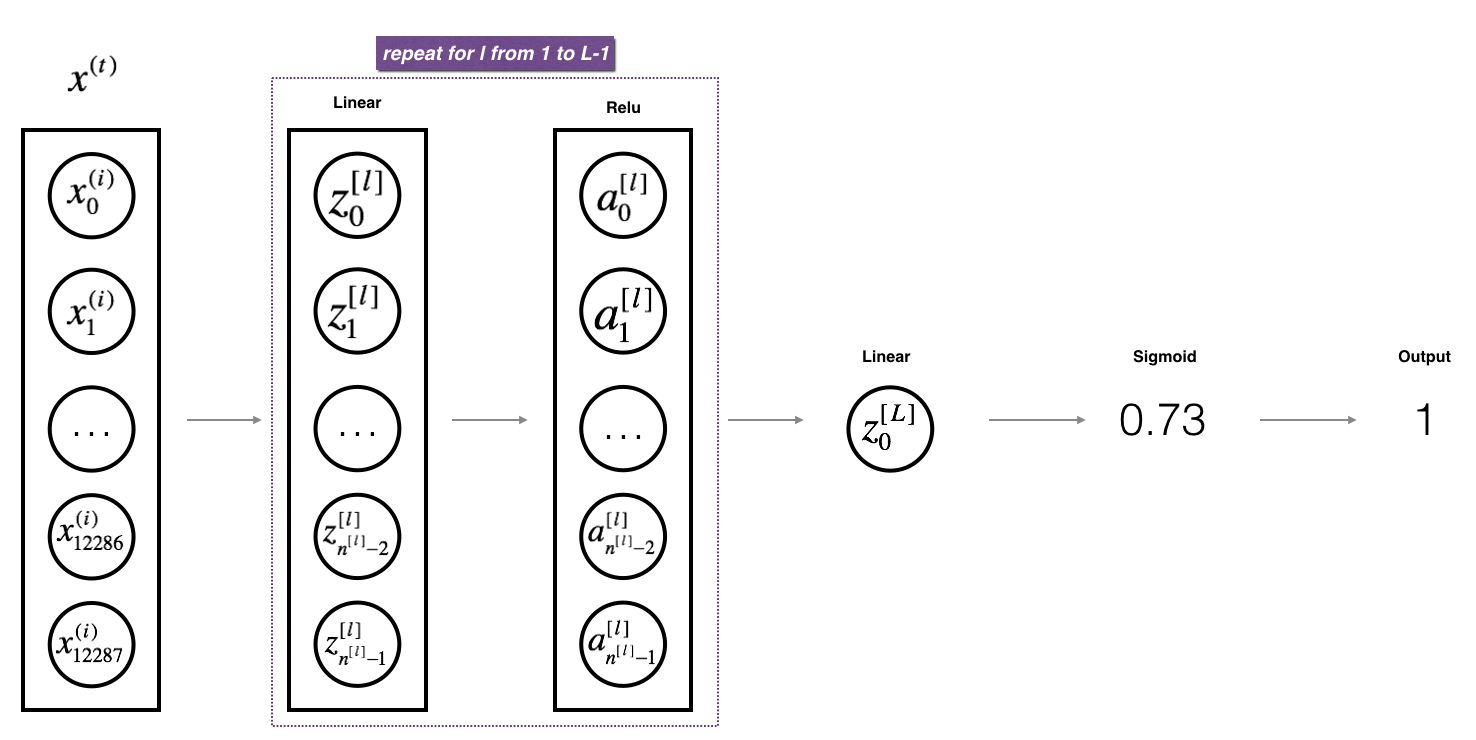
• Implement the forward propagation module (shown in purple in the figure below).  
  • Complete the LINEAR section of the layer forward propagation step (obtained)).
  • We provide you with ACTIVATION (relu / sigmoid).
  • Combine the first two steps into a new [LINEAR - > ACTIVATION] forward function.
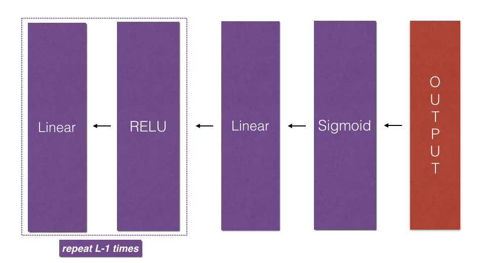
  • Stack [LINEAR - > RELU] forward function L-1 time (for Layer 1 to Layer 1) and add [LINEAR - > SIGMOID] at the end (for Layer L). This provides you with a new L_model_forward function.
• Calculate the loss.
• Implement the backward propagation module (shown in red in the figure below).  
  • Complete the LINEAR part of the layer back propagation step.
  • Let's give you the gradient of ACTIVATE function (relu_backward / sigmoid_backward)
  • Combine the first two steps into a new backward function [LINEAR - > ACTIVATION].
  • Stack back [LINEAR-> RELU] L-1 times and add back [LINEAR-> SIGMOID] in the new L_model_backward function
• Finally, the parameters are updated.

 

 

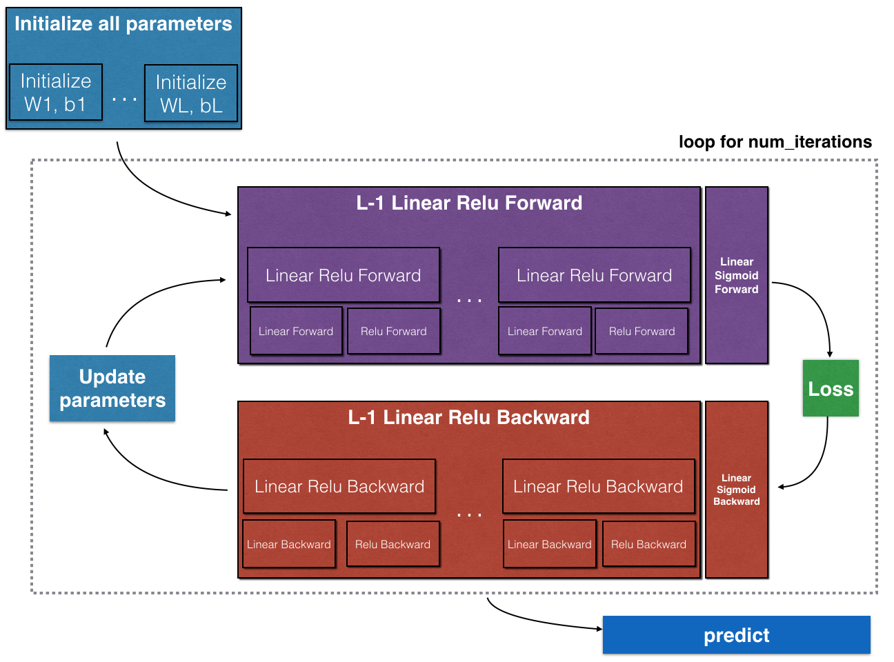
Note that for each forward function, there is a corresponding backward function. That's why at each step of the forwarding module, you store some values in the cache. Cached values are useful for calculating gradients. In the reverse propagation module, you will use the cache to calculate the gradient. This job will show you how to perform these steps.

3 - Initialization

You will write two auxiliary functions to initialize the parameters of the model. The first function will be used to initialize the parameters of the two-tier model. The second will extend this initialization process to L. layer.

3.1-2 Layer Neural Network

Exercise: Create and initialize the parameters of a two-layer neural network.

Explain:
The structure of the model is LINEAR - > RELU - > LINEAR - > SIGMOID.  
- Random initialization of weighting matrices. Use np.random.randn(shape)*0.01 for the correct shape.
- Zero initialization for deviations. Use np.zeros(shape).

def initialize_parameters(n_x,n_h,n_y):
    np.random.seed(1)

    W1=np.random.randn(n_h,n_x)*0.01
    b1=np.zeros((n_h,1))
    W2=np.random.randn(n_y,n_h)*0.01
    b2=np.zeros((n_y,1))

    assert(W1.shape==(n_h,n_x))
    assert(b1.shape==(n_h,1))
    assert(W2.shape==(n_y,n_h))
    assert(b2.shape==(n_y,1))

    parameters={"W1":W1,
    "b1":b1,
    "W2":W2,
    "b2":b2}

    return parameters

parameters = initialize_parameters(3,2,1)
print("W1 = " + str(parameters["W1"]))
print("b1 = " + str(parameters["b1"]))
print("W2 = " + str(parameters["W2"]))
print("b2 = " + str(parameters["b2"]))

3.2-L Layer Neural Network

Initialization of deeper L-layer neural networks is more complex because there are more weight matrices and bias vectors. After completion, initialize_parameters_deep, you should ensure that the dimensions of each layer match. Think back.It is the number of units in layer l. So, for example, if we enter the size of X as (12288, 209) (m=209 example) then:

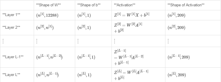
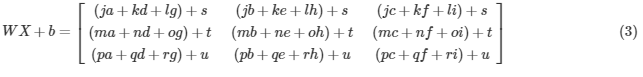
Remember, when we calculate WX + b, in python, it performs broadcasting. For example, if:

Then WX+ b will:

Exercise: Realize the initialization of L-layer neural network.

Explain:
The structure of the model is [LINEAR - > RELU] * (L-1) - > LINEAR - > SIGMOID. That is, it has an L-1 layer using ReLU activation function, followed by an output layer with sigmoid activation function.
- Random initialization of weighting matrices. Use np.random.rand(shape) * 0.01.
- Zero initialization for deviations. Use np.zeros(shape).
- We will storeThe unit number layer_dims in different layers of a variable. For example, layer_dims in last week's course "Planar Data Classification Model" is [2,4,1]: there are two inputs, one hidden layer has four hidden units, and one output layer has one output unit. Therefore, the shape of W1 is (4,2), b1 is (4,1), W2 is (1,4), and b2 is (1,1). Now you generalize this to L layer!  
This is the implementation of L=1 (single layer neural network). It should motivate you to implement the general situation (L-layer neural network).

#Initialize parameters with for loop

def initialize_parameters_deep(layer_dims):
    np.random.seed(3)
    parameters={}
    L=len(layer_dims)

    for l in range(1,L):
        parameters["W"+str(l)]=np.random.randn(layer_dims[l],layer_dims[l-1])*0.01
        parameters["b"+str(l)]=np.zeros((layer_dims[l],1))

        assert(parameters["W"+str(l)].shape==(layer_dims[l],layer_dims[l-1]))
        assert(parameters["b"+str(l)].shape==(layer_dims[l],1))
    
    return parameters
    
parameters = initialize_parameters_deep([5,4,3])
print("W1 = " + str(parameters["W1"]))
print("b1 = " + str(parameters["b1"]))
print("W2 = " + str(parameters["W2"]))
print("b2 = " + str(parameters["b2"]))

4-Forward Propagation Module

4.1 - Linear Forward

Now that you have initialized the parameters, you will propagate the forward module. You will first implement some basic functions, which you will use later when implementing the model. You will complete three functions in this order:

• LINEAR
• LINEAR - > ACTIVATION, where ACTIVATION will be ReLU or Sigmoid.
• [LINEAR - > RELU] * (L-1) - > LINEAR - > SIGMOID (whole model)

The linear forward module (vectorized in all examples) calculates the following equation:

At this time

Exercise: Construct the linear part of forward propagation.

Reminder:
The mathematical representation of the unit is. You may also find np.dot() useful. If your shapes don't match, printing W. shapes may help.

def linear_forward(A,W,b):
    Z=np.dot(W,A)+b

    assert(Z.shape==(W.shape[0],A.shape[1]))
    cache=(A,W,b)

    return Z,cache

A, W, b = linear_forward_test_case()
Z, linear_cache = linear_forward(A, W, b)
print("Z = " + str(Z))

4.2 - Linear Activated Forwarding

In this note, you will use two activation functions:

• Sigmoid: . We provide you with this sigmoid feature. This function returns two values: the activation value "a" and the cache containing "Z" (which we will input the corresponding backward function). To use it, you can call:

A, activation_cache = sigmoid(Z)

• ReLU: The mathematical formula of ReLu is A=RELU (Z) = max (0, Z). We provide you with this relu function. This function returns two values: the activation value "A" and the cache containing "Z" (this is the backward function we will input). To use it, you can call:

A, activation_cache = relu(Z)

For convenience, you will group two functions (linear and active) into one function (LINEAR - > ACTIVATION). Therefore, you will implement a function that performs the LINEAR forward step, followed by the ACTIVATION forward step.

Exercise: Realize forward propagation of LINEAR - > ACTIVATION layer. Mathematical relations are:Where the activation of "g" can be sigmoid () or relu (). Use linear_forward() and the correct activation function.

def linear_activation_forward(A_prev,W,b,activation):
    if activation=="sigmoid":
        Z,linear_cache=linear_forward(A_prev,W,b)
        A,activation_cache=sigmoid(Z)
    elif activation=="relu":
        Z,linear_cache=linear_forward(A_prev,W,b)
        A,activation_cache=relu(Z)

    assert(A.shape==(W.shape[0],A_prev.shape[1]))
    cache=(linear_cache,activation_cache)

    return A,cache

A_prev, W, b = linear_activation_forward_test_case()

A, linear_activation_cache = linear_activation_forward(A_prev, W, b, activation = "sigmoid")
print("With sigmoid: A = " + str(A))

A, linear_activation_cache = linear_activation_forward(A_prev, W, b, activation = "relu")
print("With ReLU: A = " + str(A))

Note: In deep learning, "[LINEAR-> ACTIVATION]" calculation is counted as a single layer rather than two layers in the neural network.

d) L-Layer Model

In order to implement L-layer neural networks more conveniently, you need to copy the function L-1 of the previous (linear_activation_forward using RELU) and then use the SIGMOID function of linear_activation_forward.

Exercise: Realize the forward propagation of the above model.

Description: In the following code, the variable AL will representThis is the case. (This is sometimes called Yhat, or Yhat.)

Tips:
- Use the functions you wrote earlier
- Replicate [LINEAR-> RELU] (L-1) times using for loop
- Don't forget to track caches in the Cache list. To add a list with a new value c, you can use list.append(c).

def L_model_forward(X,parameters):
    caches=[]
    A=X
    L=len(parameters)//2 "/" Dividing down
    
    for l in range(1,L):
        A_prev=A
        A,cache=linear_activation_forward(A_prev,parameters["W"+str(l)],parameters["b"+str(l)],"relu")
        caches.append(cache)
            
    AL,cache=linear_activation_forward(A,parameters["W"+str(L)],parameters["b"+str(L)],"sigmoid")
    caches.append(cache)

    assert(AL.shape==(1,X.shape[1]))

    return AL,caches

X, parameters = L_model_forward_test_case_2hidden()
AL, caches = L_model_forward(X, parameters)
print("AL = " + str(AL))
print("Length of caches list = " + str(len(caches)))

Now you have a complete forward propagation, which accepts input X and outputs a row vector.Include your prediction. It also records all intermediate values in the cache. UseYou can calculate the estimated cost.

5-Cost Function

Now, you will achieve forward and backward propagation. You need to calculate the cost, because you need to check whether your model actually learns.

Exercise: Calculate cross-entropy cost J, using the following formula:

def compute_cost(AL,Y):
    m=Y.shape[1]

    cost=-np.sum(np.multiply(np.log(AL),Y)+np.multiply(np.log(1-AL),1-Y))/m

    cost=np.squeeze(cost)
    assert(cost.shape==())
    
    return cost

Y, AL = compute_cost_test_case()

print("cost = " + str(compute_cost(AL, Y)))

6 - Backward Propagation Module

Just like forward propagation, you will implement auxiliary functions for back propagation. Keep in mind that back propagation is used to calculate the gradient of the loss function relative to the parameter.

Reminder:

 

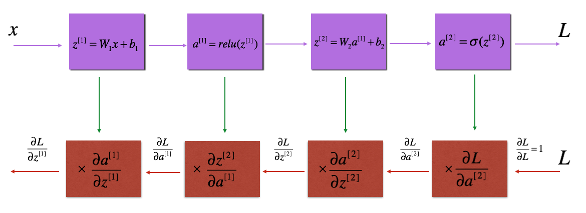
Figure 3: Forward and backward propagation of LINEAR - > RELU - > LINEAR - > SIGMOID
Purple blocks represent forward propagation, and red blocks represent backward propagation.

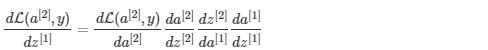
To calculate the gradientYou use the old chain ruleThis is the case. During reverse propagation, in each step, the current gradient is multiplied by the gradient corresponding to a particular layer to obtain the required gradient. Equivalently, in order to calculate the gradientYou use the old chain ruleThis is the case. That's why we talk about "back propagation".

Now, similar to forward propagation, you will build backward propagation in three steps:
- Backward linearity

- LINEAR - > ACTIVATION, calculating the derivatives of ReLU or sgmoid activation functions
- [LINEAR - > RELU] * (L-1) - > LINEAR - > SIGMOID backward propagation (whole model)

6.1 - Linear Backward

For Layer 1, the l inear part is:(Then the activation function).

Suppose you have calculated the derivative.This is the case. You can imagine ().

Three outputs ((by input)Calculated, this is the formula you need:

Exercise: Use the three formulas above to implement linear_backward ().

def linear_backward(dZ,cache):
    A_prev,W,b=cache
    m=A_prev.shape[1]

    dW=np.dot(dZ,A_prev.T)/m
    db=np.sum(dZ,axis=1,keepdims=True)/m
    dA_prev=np.dot(W.T,dZ)

    assert(dA_prev.shape==A_prev.shape)
    assert(dW.shape==W.shape)
    assert(db.shape==b.shape)

    return dA_prev,dW,db

dZ, linear_cache = linear_backward_test_case()

dA_prev, dW, db = linear_backward(dZ, linear_cache)
print ("dA_prev = "+ str(dA_prev))
print ("dW = " + str(dW))
print ("db = " + str(db))

6.2 - Backward linear activation

Next, you will create a function that combines two auxiliary functions: linear_backward and the back step of activation, linear_activation_backward.

To help you implement linear_activation_backward, we provide two backward functions:
sigmoid_backward: Backward propagation for SIGMOID cells. You can call it as follows:

dZ = sigmoid_backward(dA, activation_cache)

- relu_backward: To achieve the reverse propagation of RELU units. You can call it as follows:

dZ = relu_backward(dA, activation_cache)

If g(.) is the activation function, sigmoid_backward and relu_backward are calculated.

Exercise: Realize reverse propagation of LINEAR - > ACTIVATION layer.

def linear_activation_backward(dA,cache,activation):
    linear_cache,activation_cache=cache

    if activation=="relu":
        dZ=relu_backward(dA,activation_cache)
        dA_prev,dW,db=linear_backward(dZ,linear_cache)
    elif activation=="sigmoid":
        dZ=sigmoid_backward(dA,activation_cache)
        dA_prev,dW,db=linear_backward(dZ,linear_cache)

    return dA_prev,dW,db

AL, linear_activation_cache = linear_activation_backward_test_case()

dA_prev, dW, db = linear_activation_backward(AL, linear_activation_cache, activation = "sigmoid")
print ("sigmoid:")
print ("dA_prev = "+ str(dA_prev))
print ("dW = " + str(dW))
print ("db = " + str(db) + "\n")

dA_prev, dW, db = linear_activation_backward(AL, linear_activation_cache, activation = "relu")
print ("relu:")
print ("dA_prev = "+ str(dA_prev))
print ("dW = " + str(dW))
print ("db = " + str(db))

6.3-L Model Backward

Now, you will implement backward functionality for the entire network. Recall that when you implement the L_model_forward function, you store a cache containing (X, W, b and z) at each iteration. In the reverse propagation module, you will use these variables to calculate the gradient. Therefore, in the L_model_backward function, you will traverse all hidden layers back from layer L. In each step, you will use layer 1 cache escalation to propagate back through layer L. Figure 5 below shows backward propagation.

* Initialize backpropagation*:
To propagate backwards through this network, we know that the output is uuuuuuuuuuuThis is the case. Therefore, your code needs to be computedThis is the case. For this purpose, please use this formula (using calculus derivations that you do not need to know more about):

dAL = - (np.divide(Y, AL) - np.divide(1 - Y, 1 - AL)) 

Then, you can use this activated gradient dAL to move on. As shown in Figure 5, you can now dAL input the LINEAR - > SIGMOID backward function you implemented (which will use the cache value stored by the L_model_forward function). Later, you will have to use the for loop to iterate through all other layers using the LINEAR - > RELU backward function. You should store each dA, dW, and db in the grads dictionary. To this end, use the following formula:

For example, for l=3, it will be stored inIn grads["dW3"].

Exercise: To implement the back propagation [LINEAR - > RELU] * (L-1) - > LINEAR - > SIGMOID model.

def L_model_backward(AL,Y,caches):
    grads={}
    L=len(caches)
    m=AL.shape[1]
    Y=Y.reshape(AL.shape)
    
    dAL=-(np.divide(Y,AL)-np.divide(1-Y,1-AL))

    current_cache=caches[L-1]
    grads["dA"+str(L)],grads["dW"+str(L)],grads["db"+str(L)]=linear_activation_backward(dAL,current_cache,"sigmoid")

    for l in reversed(range(L-1)):
        current_cache=caches[l]
        dA_prev_temp,dW_temp,db_temp=linear_activation_backward(grads["dA"+str(l+2)],current_cache,"relu")
        grads["dA"+str(l+1)]=dA_prev_temp
        grads["dW"+str(l+1)]=dW_temp
        grads["db"+str(l+1)]=db_temp

    return grads

AL, Y_assess, caches = L_model_backward_test_case()
grads = L_model_backward(AL, Y_assess, caches)
print_grads(grads)

6.4 - Update parameters

In this section, you will update the parameters of the model using gradient descent:

One of them is the learning rate. After calculating the updated parameters, they are stored in the parameter dictionary.

Exercise: update_parameters() uses gradient descent to update parameters.

Explain:
Use gradient descent updates on each W and b.

def update_parameters(parameters,grads,learning_rate):
    L=len(parameters)//2

    for l in range(L):
        parameters["W"+str(l+1)]=parameters["W"+str(l+1)]-learning_rate*grads["dW"+str(l+1)]
        parameters["b"+str(l+1)]=parameters["b"+str(l+1)]-learning_rate*grads["db"+str(l+1)]

    return parameters

parameters, grads = update_parameters_test_case()
parameters = update_parameters(parameters, grads, 0.1)

print ("W1 = "+ str(parameters["W1"]))
print ("b1 = "+ str(parameters["b1"]))
print ("W2 = "+ str(parameters["W2"]))
print ("b2 = "+ str(parameters["b2"]))

7 - Conclusion

Congratulations on all the functions needed to build a deep neural network!

We know it's a long task, but progress will only get better. The next part of the allocation is easier.

In the next task, you will combine all of these to build two models:
- Bilevel Neural Network
- L-Layer Neural Network

In fact, you will use these models to classify cat and non-cat images!