1: Boston house price forecast task
In the previous section, we have a preliminary understanding of the basic concepts of neural networks (such as neurons, multi-layer connections, forward computing, calculation charts) and three elements of model structure (model hypothesis, evaluation function and optimization algorithm). This section will take the Boston house price task as an example to introduce the thinking process and operation method of building neural network model using Python language and Numpy library.
Boston house price forecasting is a classic machine learning task, similar to the "Hello World" of the programmer world. As we all know about house price, the house price in Boston area is influenced by many factors. This data set counts 13 factors that may affect the house price and the average price of this type of house. It is expected to build a model for house price prediction based on 13 factors, as shown in Figure 1.
Figure 1: schematic diagram of influencing factors of house price in Boston
For the prediction problem, it can be divided into regression task and classification task according to whether the type of prediction output is continuous real value or discrete label. Because house price is a continuous value, house price prediction is obviously a regression task. Next we try to use the simplest linear regression model to solve this problem, and use neural network to realize this model.
1: Linear regression model
It is assumed that the relationship between the house price and the influencing factors can be described in a linear way:
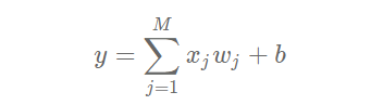
The solution of the model is to fit each w and b by data. wj and b represent the weight and bias of the linear model respectively. In one-dimensional case, wj and b are the slope and intercept of the line.
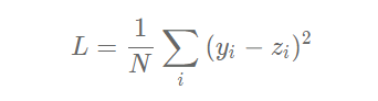
The linear regression model uses the mean square error as the Loss function to measure the difference between the predicted house price and the real house price. The formula is as follows: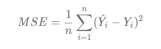
reflection:
Why use mean square error as loss function? That is to say, the prediction error of the model on each training sample is added to measure the accuracy of the whole sample. This is because the design of loss function not only needs to consider "rationality", but also needs to consider "solvability". This problem will be elaborated in the later content.
2: Neural network structure of linear regression model
In the standard structure of neural network, each neuron is composed of weighted sum and nonlinear transformation, and then multiple neurons are placed in layers and connected to form neural network. The linear regression model can be considered as a very simple special case of the neural network model. It is a neuron with only weighted sum and no nonlinear transformation (no need to form a network), as shown in Figure 2.
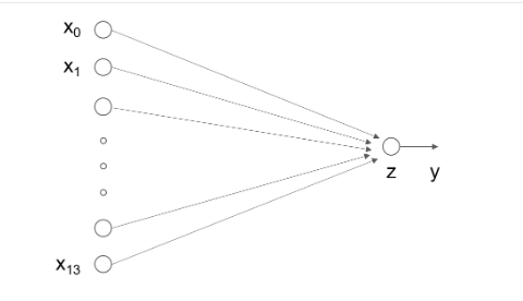
Figure 2: neural network structure of linear regression model
2: Building the neural network model of Boston house price forecasting task
Deep learning not only realizes the end-to-end learning of the realization model, but also promotes the AI to enter the stage of industrial production, resulting in a general framework of standardization, automation and modularization. The in-depth learning model of different scenes has certain universality. The model can be constructed and trained in five steps, as shown in Figure 3.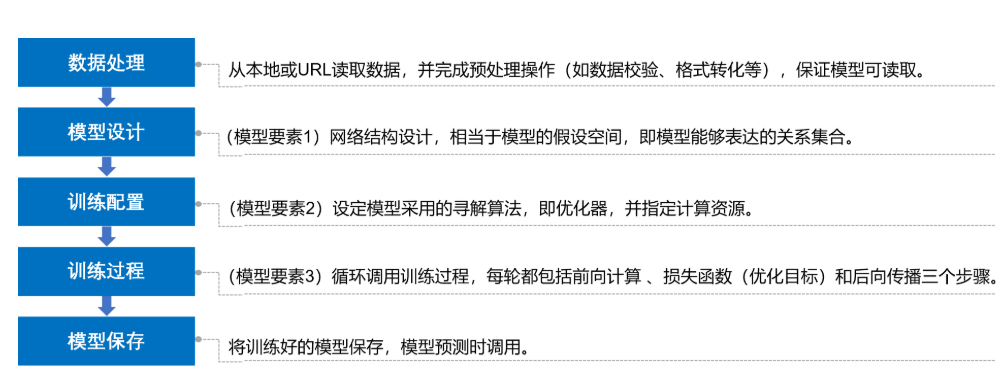
Figure 3: basic steps of building neural network / deep learning model
Because of the universality of the modeling and training process of deep learning, when building different models, only when the three elements of the model are different and the other steps are basically the same, can the deep learning framework be used.
1: Data processing
Data processing includes five parts: data import, data shape transformation, data set partition, data normalization and encapsulation of load data function. Data can only be called by the model after preprocessing.
explain:
The code in this tutorial can be run directly on AIStudio, and the Print results are based on the actual running results of the program.
As it is a real case, there is a dependency before the code, so readers need to run it one by one, or Print will report an error.
2: Read in data
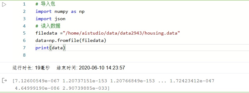
Read in the data through the following code to understand the data set structure of Boston house prices. The data is stored in the local directory housing.data File.
# Import package
import numpy as np
import json
# read in data
filedata ="/home/aistudio/data/data2943/housing.data"
data=np.fromfile(filedata)
print(data)
3: Data shape transformation
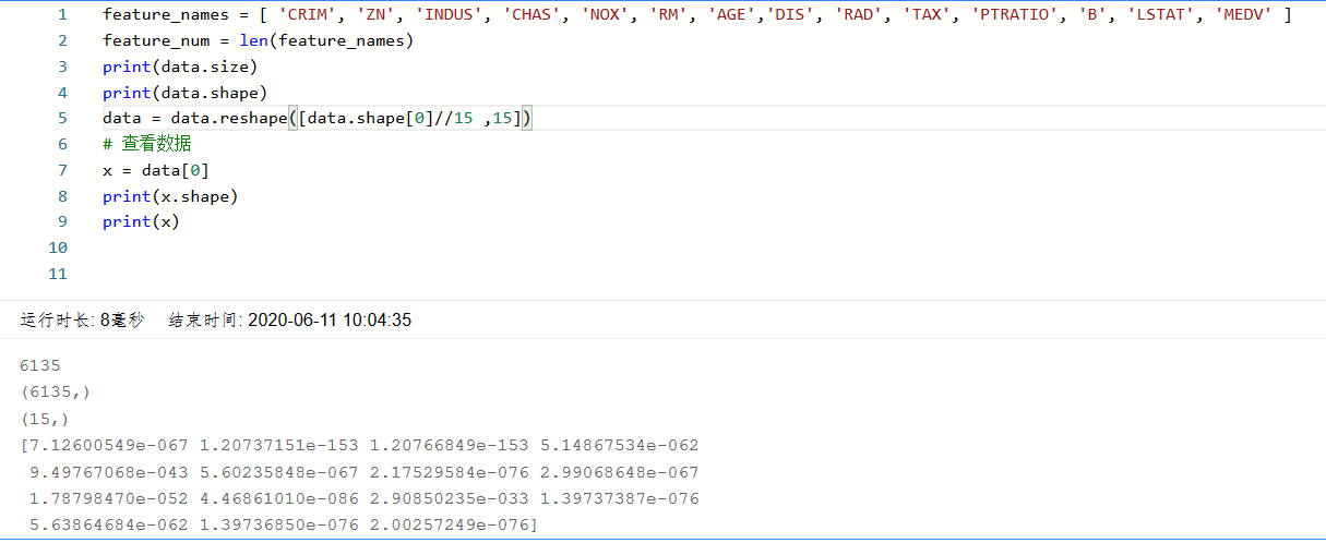
Since the original data read in is one-dimensional, all the data are connected together. Therefore, we need to transform the shape of the data to form a two-dimensional matrix. Each row of data samples (14 values), each data sample contains 13 X (characteristics affecting house price) and a Y (average price of this type of house).
# After reading in, the data is converted into 1-D array, in which 0-13 items of array are the first data, 14-27 items are the second data, and so on
# Here, reshape the original data into the form of N x 14
feature_names = [ 'CRIM', 'ZN', 'INDUS', 'CHAS', 'NOX', 'RM', 'AGE','DIS',
                 'RAD', 'TAX', 'PTRATIO', 'B', 'LSTAT', 'MEDV' ]
feature_num = len(feature_names)
data = data.reshape([data.shape[0] // feature_num, feature_num])
# View data
x = data[0]
print(x.shape)
print(x)
4: Dataset partition
The data set is divided into training set and test set, in which the training set is used to determine the parameters of the model, and the test set is used to evaluate the effect of the model. Why do you want to split the dataset and not directly apply it to model training? This is similar to the relationship between teaching and examination in the student era, as shown in Figure 4.
Figure 4: significance of splitting training set and test set
At school, there are always some smart students who don't study hard at ordinary times. Before the exam, they cram the exercises by rote, but the results are often not good. Because the school expects students to master knowledge, not just the exercises themselves. Another new examination questions can encourage students to master the principles behind the exercises. We also expect the model to learn the essence of the task, not the training data itself. Only the unused data of the model training can more truly evaluate the effect of the model.
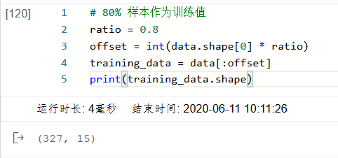
In this case, we use 80% of the data as training set and 20% as test set. The implementation code is as follows. By printing the shape of the training set, we can find that there are 404 samples, each of which contains 13 features and 1 prediction value.
ratio = 0.8
offset = int(data.shape[0] * ratio)
training_data = data[:offset]
training_data.shape
5: Data normalization
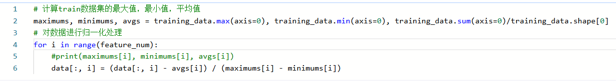
Each feature is normalized so that the value of each feature is scaled to 0 ~ 1. There are two advantages: one is that the model training is more efficient; the other is that the weight before the feature can represent the contribution of the variable to the prediction results (because the range of each feature value itself is the same).
# Calculate the maximum, minimum and average value of the train data set
maximums, minimums, avgs = training_data.max(axis=0), training_data.min(axis=0), training_data.sum(axis=0)/training_data.shape[0]
# Normalize the data
for i in range(feature_num):
	#print(maximums[i], minimums[i], avgs[i])
	data[:, i] = (data[:, i] - avgs[i]) / (maximums[i] - minimums[i])
6: : encapsulated as load data function
Encapsulate the above data processing operations into the load data function for the next model call. The code is as follows.
def load_data():
    # Import data from file
    datafile = './work/housing.data'
    data = np.fromfile(datafile, sep=' ')

    # Each data includes 14 items, of which the first 13 items are the influencing factors, and the 14th item is the corresponding median housing price
    feature_names = [ 'CRIM', 'ZN', 'INDUS', 'CHAS', 'NOX', 'RM', 'AGE', \
                      'DIS', 'RAD', 'TAX', 'PTRATIO', 'B', 'LSTAT', 'MEDV' ]
    feature_num = len(feature_names)

    # Reshape the original data to a shape like [N, 14]
    data = data.reshape([data.shape[0] // feature_num, feature_num])

    # Split the original data set into training set and test set
    # 80% of the data is used for training and 20% for testing
    # There must be no intersection between test set and training set
    ratio = 0.8
    offset = int(data.shape[0] * ratio)
    training_data = data[:offset]

    # Calculate the maximum, minimum and average value of the train data set
    maximums, minimums, avgs = training_data.max(axis=0), training_data.min(axis=0), \
                                 training_data.sum(axis=0) / training_data.shape[0]

    # Normalize the data
    for i in range(feature_num):
        #print(maximums[i], minimums[i], avgs[i])
        data[:, i] = (data[:, i] - avgs[i]) / (maximums[i] - minimums[i])

    # Partition ratio of training set and test set
    training_data = data[:offset]
    test_data = data[offset:]
    return training_data, test_data
# get data
training_data, test_data = load_data()
x = training_data[:, :-1]
y = training_data[:, -1:]
# View data
print(x[0])
print(y[0])
[-0.02146321  0.03767327 -0.28552309 -0.08663366  0.01289726  0.04634817
  0.00795597 -0.00765794 -0.25172191 -0.11881188 -0.29002528  0.0519112
 -0.17590923]
[-0.00390539]
7: Model design
Model design is one of the key elements of deep learning model, also known as network structure design, which is equivalent to the assumption space of the model, that is, the process of "forward calculation" (from input to output) of the model.
If the input feature and the output predicted value are represented by vectors, the input feature x has 13 components and y has 1 component, then the shape of the parameter weight is 13 × 1. Suppose we initialize with any of the following numeric assignment parameters:

w = [0.1, 0.2, 0.3, 0.4, 0.5, 0.6, 0.7, 0.8, -0.1, -0.2, -0.3, -0.4, 0.0]
w = np.array(w).reshape([13, 1])
Take out the first sample data and observe the result of multiplying the eigenvector and the parameter vector of the sample.
x1=x[0]
t = np.dot(x1, w)
print(t)
[0.03395597]
For a complete linear regression formula, the offset bbb should also be initialized, and the initial value of - 0.2 should also be assigned at will. Then, the complete output of linear regression model is z=t+bz=t+bz=t+b. this process of calculating output value from characteristics and parameters is called "forward calculation".
b = -0.2
z = t + b
print(z)
[-0.16604403]
The above process of calculating the predicted output is described in the way of "class and object". The class member variables include the parameters www and bbb. Write a forward function (for "forward calculation") to complete the above calculation process from features and parameters to output predicted value. The code is as follows.
class Network(object):
    def __init__(self, num_of_weights):
        # Initial value of randomly generated w
        # In order to maintain the consistency of the results of each run of the program,
        # Set fixed random number seed here
        np.random.seed(0)
        self.w = np.random.randn(num_of_weights, 1)
        self.b = 0.

    def forward(self, x):
        z = np.dot(x, self.w) + self.b
        return z
Based on the definition of Network class, the calculation process of the model is as follows.
net = Network(13)
x1 = x[0]
y1 = y[0]
z = net.forward(x1)
print(z)
[-0.63182506]
8: Training configuration
After the completion of the model design, it is necessary to find the optimal value of the model through the training configuration, that is, to measure the quality of the model through the loss function. Training configuration is also one of the key elements of deep learning model.
Calculate x1 by model
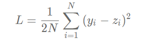
The house price corresponding to the influencing factors indicated should be zzz, but the actual data tells us that the house price is yyy. At this time, we need some indicators to measure the gap between the predicted value zzz and the real value yyy. For the regression problem, the most commonly used measurement method is to use the mean square error as the index to evaluate the quality of the model. The specific definition is as follows:

The Loss (L) in the above formula is also known as Loss function, which is an indicator to measure the quality of the model. In the regression problem, the mean square error is a common form. In the classification problem, the cross entropy is usually used as the Loss function, which will be introduced in more detail in the following chapters. The code to calculate the Loss of a sample is as follows:
Loss = (y1 - z)*(y1 - z)
print(Loss)
[0.39428312]
Because the loss of each sample needs to be taken into account when calculating the loss, we need to sum the loss function of a single sample and divide it by the total number of samples N.
The calculation process of adding loss function under Network class is as follows:
class Network(object):
    def __init__(self, num_of_weights):
        # Initial value of randomly generated w
        # In order to maintain the consistency of the results of each run of the program, a fixed random number seed is set here
        np.random.seed(0)
        self.w = np.random.randn(num_of_weights, 1)
        self.b = 0.

    def forward(self, x):
        z = np.dot(x, self.w) + self.b
        return z

    def loss(self, z, y):
        error = z - y
        cost = error * error
        cost = np.mean(cost)
        return cost
Using the defined Network class, it is convenient to calculate the prediction value and loss function. It should be noted that the variables xxx, www, BBB, zzz, errorerrorror in the class are all vectors. Take the variable xxx as an example. There are two dimensions in total. One represents the characteristic quantity (value is 13) and the other represents the sample quantity. The code is as follows.
net = Network(13)
# Here, the prediction value and loss function of multiple samples can be calculated at one time
x1 = x[0:3]
y1 = y[0:3]
z = net.forward(x1)
print('predict: ', z)
loss = net.loss(z, y1)
print('loss:', loss)
predict:  [[-0.63182506]
 [-0.55793096]
 [-1.00062009]]
loss: 0.7229825055441156
9: Training process
The above calculation process describes how to build a neural network, through which the prediction value and Loss function are calculated. Next, it introduces how to solve the numerical value of parameters w and b, which is also called model training process. The training process is one of the key elements of the deep learning model, whose goal is to make the Loss function defined as small as possible, that is to find a parameter solution W and b to make the Loss function get the minimum value.
Let's do a small test first: as shown in Figure 5, based on the knowledge of calculus, find out that the slope of a curve at a certain point is equal to the derivative value of the function at that point. So let's think about the slope at the extreme point of the curve?
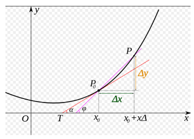
Figure 5: curve slope equal to derivative
This question is not difficult to answer. The slope at the extreme point of the curve is 0, that is, the derivative of the function at the extreme point is 0. Then, www and bbb, which minimize the loss function, should be the solutions of the following equations:
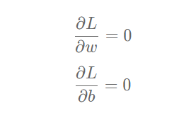
The values of www and bbb can be obtained by introducing sample data (x,y)(x, y)(x,y) into the above equations, but this method is only effective for simple tasks such as linear regression. If the model contains nonlinear transformation, or the loss function is not a simple form of mean square deviation, it is difficult to solve by the above formula. In order to solve this problem, we will introduce a more general numerical method: gradient descent method.
10: Gradient descent method
In reality, there are a lot of functions which are easy to be solved in the forward direction and difficult to be solved in the reverse direction. This function has a lot of applications in cryptography. The characteristic of cryptographic lock is that it can quickly judge whether a key is correct (knowing x, finding y is easy), but even if we get the cryptographic lock system, we can't find out what the correct key is (knowing y, finding x is difficult).
This situation is particularly similar to a blind man who wants to walk from the mountain to the valley. He can't see where the valley is (he can't find the parameter value of $Loss when the derivative is 0), but he can stretch his foot to explore the slope around him (the derivative value of the current point, also known as gradient). Then, the solution of the minimum value of Loss function can be realized by "taking the value of current parameter, descending step by step in the direction of downhill until reaching the lowest point". This method I personally call it "blind downhill method". Oh no, there's a more formal term for "gradient descent".
The key of training is to find a set of (w,b) to minimize the loss function LLL. Let's first look at the loss function L with only two parameters w5
The simple situation of change, inspired by the idea of finding solutions.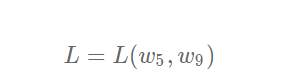

net = Network(13)
losses = []
#Only the curve parts of parameters w5 and w9 in the interval [- 160, 160] and the extremum containing loss function are drawn
w5 = np.arange(-160.0, 160.0, 1.0)
w9 = np.arange(-160.0, 160.0, 1.0)
losses = np.zeros([len(w5), len(w9)])

#Calculate the Loss corresponding to each parameter value in the setting area
for i in range(len(w5)):
    for j in range(len(w9)):
        net.w[5] = w5[i]
        net.w[9] = w9[j]
        z = net.forward(x)
        loss = net.loss(z, y)
        losses[i, j] = loss

#Use matplotlib to make 3dgraph of two variables and corresponding Loss
import matplotlib.pyplot as plt
from mpl_toolkits.mplot3d import Axes3D
fig = plt.figure()
ax = Axes3D(fig)

w5, w9 = np.meshgrid(w5, w9)

ax.plot_surface(w5, w9, losses, rstride=1, cstride=1, cmap='rainbow')
plt.show()
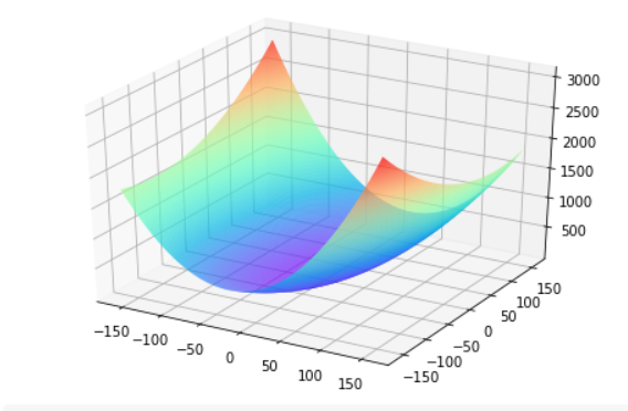
It needs to be explained: why do we choose w5 and w9 to draw here? This is because when choosing these two parameters, we can find the existence of extremum on the surface graph of loss function intuitively. For other parameter combinations, it is not intuitive to observe the extreme point of loss function from the graph.
It is one of the reasons why we choose the mean square error as the loss function. Figure 6 shows the loss function curve of mean square error and absolute value error (only the error of each sample is accumulated, not the square processing) when there is only one parameter dimension.
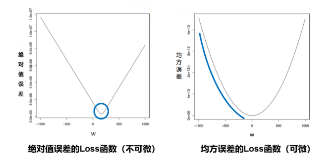
Figure 6: curve of mean square error and absolute value error loss function
Thus, the "smooth" slope represented by mean square error has two advantages:
- The lowest point of the curve is differentiable.
- The closer to the lowest point, the slope of the curve slows down gradually, which helps to judge the degree of approaching the lowest point based on the current gradient (whether to gradually reduce the step size to avoid missing the lowest point).
However, the absolute value errors of these two characteristics are not available, which is also the reason why the design of loss function should not only consider "rationality", but also pursue "easiness".
Now we need to find a set of values of [w5,w9] to minimize the loss function. The scheme to realize gradient descent method is as follows:
- Step 1: randomly select a set of initial values, for example: [w5,w9] = [− 100.0, − 100.0]
- Step 2: select the next point [w5 ′, w9 ′], so that L(w5 ′, w9 ′) < L(w5, w9)
- Step 3: repeat step 2 until the loss function almost no longer drops.
How to choose [w5 ′, w9 ′] is very important. The first is to ensure that L is declining, and the second is to make the declining trend as fast as possible. The basic knowledge of calculus tells us that along the reverse direction of the gradient, it is the direction in which the function value drops the fastest, as shown in Figure 7. It is easy to understand that the gradient direction of a function at a certain point is the direction with the largest slope of the curve, but the gradient direction is upward, so the reverse direction of the gradient is the fastest to decline.
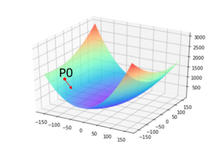
Figure 7: schematic diagram of gradient descent direction
11: Calculation gradient
We have talked about the calculation method of loss function above, which is slightly rewritten here. In order to simplify the gradient calculation, factor 1 / 2 is introduced
, define the loss function as follows:
Where zi is the prediction value of the network for the ith sample:
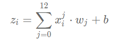
Definition of gradient:
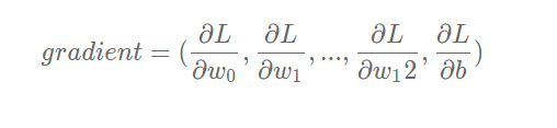
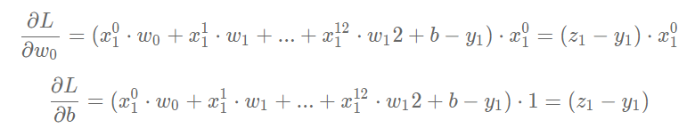
The partial derivatives of LLL to www and bbb can be calculated:
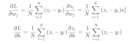
It can be seen from the calculation process of derivative that factor 1 / 2 is eliminated, because factor 222 will be generated when derivative of quadratic function is calculated, which is also the reason why we rewrite the loss function.
Let's consider the gradient calculation when there is only one sample:
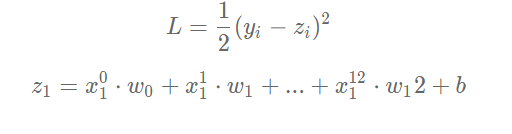
The partial derivatives of L to w and b can be calculated:
You can view the data and dimensions of each variable through a specific program.
x1 = x[0]
y1 = y[0]
z1 = net.forward(x1)
print('x1 {}, shape {}'.format(x1, x1.shape))
print('y1 {}, shape {}'.format(y1, y1.shape))
print('z1 {}, shape {}'.format(z1, z1.shape))
x1 [-0.02146321  0.03767327 -0.28552309 -0.08663366  0.01289726  0.04634817
  0.00795597 -0.00765794 -0.25172191 -0.11881188 -0.29002528  0.0519112
 -0.17590923], shape (13,)
y1 [-0.00390539], shape (1,)
z1 [-12.05947643], shape (1,)
According to the above formula, when there is only one sample, the gradient of a certain wj, such as w0, can be calculated.
gradient_w0 = (z1 - y1) * x1[0]
print('gradient_w0 {}'.format(gradient_w0))
gradient_w0 [0.25875126]
Again, we can calculate the gradient of w1.
gradient_w1 = (z1 - y1) * x1[1]
print('gradient_w1 {}'.format(gradient_w1))
gradient_w1 [-0.45417275]
The gradient of w2 is calculated in turn.
gradient_w2= (z1 - y1) * x1[2]
print('gradient_w1 {}'.format(gradient_w2))
gradient_w1 [3.44214394]
Smart readers may have thought that writing a for loop can calculate the gradient of all weights from w0 to w12, which can be implemented by readers themselves.
12: Gradient calculation with Numpy
Based on the Numpy broadcast mechanism (the calculation of vector and matrix is the same as that of a single variable), the gradient calculation can be realized more quickly. In the code of gradient calculation, we directly use (z1 - y1) * x1 to get a 13 dimensional vector, and each component represents the gradient of the dimension.
gradient_w = (z1 - y1) * x1
print('gradient_w_by_sample1 {}, gradient.shape {}'.format(gradient_w, gradient_w.shape))
gradient_w_by_sample1 [ 0.25875126 -0.45417275  3.44214394  1.04441828 -0.15548386 -0.55875363
 -0.09591377  0.09232085  3.03465138  1.43234507  3.49642036 -0.62581917
  2.12068622], gradient.shape (13,)
There are multiple samples in the input data, each of which contributes to the gradient. The above code calculates the gradient value when only sample 1 is available. The same calculation method can also calculate the contribution of sample 2 and sample 3 to the gradient.
x2 = x[1]
y2 = y[1]
z2 = net.forward(x2)
gradient_w = (z2 - y2) * x2
print('gradient_w_by_sample2 {}, gradient.shape {}'.format(gradient_w, gradient_w.shape))
gradient_w_by_sample2 [ 0.7329239   4.91417754  3.33394253  2.9912385   4.45673435 -0.58146277
 -5.14623287 -2.4894594   7.19011988  7.99471607  0.83100061 -1.79236081
  2.11028056], gradient.shape (13,)
x3 = x[2]
y3 = y[2]
z3 = net.forward(x3)
gradient_w = (z3 - y3) * x3
print('gradient_w_by_sample3 {}, gradient.shape {}'.format(gradient_w, gradient_w.shape))
gradient_w_by_sample3 [ 0.25138584  1.68549775  1.14349809  1.02595515  1.5286008  -1.93302947
  0.4058236  -0.85385157  2.46611579  2.74208162  0.28502219 -0.46695229
  2.39363651], gradient.shape (13,)
Some readers may think again that they can use the for loop to calculate the contribution of each sample to the gradient, and then average it. But we don't need to do this. We can still use Numpy's matrix operation to simplify the operation, such as in the case of three samples.
# Note that this is the data of three samples at a time, not the third sample
x3samples = x[0:3]
y3samples = y[0:3]
z3samples = net.forward(x3samples)

print('x {}, shape {}'.format(x3samples, x3samples.shape))
print('y {}, shape {}'.format(y3samples, y3samples.shape))
print('z {}, shape {}'.format(z3samples, z3samples.shape))
x [[-0.02146321  0.03767327 -0.28552309 -0.08663366  0.01289726  0.04634817
   0.00795597 -0.00765794 -0.25172191 -0.11881188 -0.29002528  0.0519112
  -0.17590923]
 [-0.02122729 -0.14232673 -0.09655922 -0.08663366 -0.12907805  0.0168406
   0.14904763  0.0721009  -0.20824365 -0.23154675 -0.02406783  0.0519112
  -0.06111894]
 [-0.02122751 -0.14232673 -0.09655922 -0.08663366 -0.12907805  0.1632288
  -0.03426854  0.0721009  -0.20824365 -0.23154675 -0.02406783  0.03943037
  -0.20212336]], shape (3, 13)
y [[-0.00390539]
 [-0.05723872]
 [ 0.23387239]], shape (3, 1)
z [[-12.05947643]
 [-34.58467747]
 [-11.60858134]], shape (3, 1)
The first dimension of x3samples, y3samples and z3samples above is 3, indicating that there are 3 samples. The contribution of these three samples to the gradient is calculated below.
gradient_w = (z3samples - y3samples) * x3samples
print('gradient_w {}, gradient.shape {}'.format(gradient_w, gradient_w.shape))
gradient_w [[ 0.25875126 -0.45417275  3.44214394  1.04441828 -0.15548386 -0.55875363
  -0.09591377  0.09232085  3.03465138  1.43234507  3.49642036 -0.62581917
   2.12068622]
 [ 0.7329239   4.91417754  3.33394253  2.9912385   4.45673435 -0.58146277
  -5.14623287 -2.4894594   7.19011988  7.99471607  0.83100061 -1.79236081
   2.11028056]
 [ 0.25138584  1.68549775  1.14349809  1.02595515  1.5286008  -1.93302947
   0.4058236  -0.85385157  2.46611579  2.74208162  0.28502219 -0.46695229
   2.39363651]], gradient.shape (3, 13)
As you can see here, calculate gradient_ The dimension of W is 3 × 13, and the gradient calculated by the first line and the first sample above is gradient_w_by_sample1 is consistent, and the second line is the gradient calculated by the second sample above_ W_ By_ Sample1 is the same, and the third line is the gradient calculated by the third sample above_ W_ By_ Sample1 is consistent. Using matrix operation, it is more convenient to calculate the contribution of each sample to the gradient.
In the case of N samples, we can directly use the following method to calculate the contribution of all samples to the gradient, which is the convenience of using the Numpy library broadcast function. To summarize, the broadcast function of Numpy library is used here:
-
On the one hand, the dimension of parameters can be extended to calculate the gradient of all parameters from w0 to w12 for one sample instead of for loop.
-
On the other hand, we can extend the dimension of samples, instead of for loop, to calculate the gradient of sample 0 to sample 403.
  z = net.forward(x)
  gradient_w = (z - y) * x
  print('gradient_w shape {}'.format(gradient_w.shape))
  print(gradient_w)
  gradient_w shape (404, 13)
  [[  0.25875126  -0.45417275   3.44214394 ...   3.49642036  -0.62581917
      2.12068622]
   [  0.7329239    4.91417754   3.33394253 ...   0.83100061  -1.79236081
      2.11028056]
   [  0.25138584   1.68549775   1.14349809 ...   0.28502219  -0.46695229
      2.39363651]
   ...
   [ 14.70025543 -15.10890735  36.23258734 ...  24.54882966   5.51071122
     26.26098922]
   [  9.29832217 -15.33146159  36.76629344 ...  24.91043398  -1.27564923
     26.61808955]
   [ 19.55115919 -10.8177237   25.94192351 ...  17.5765494    3.94557661
     17.64891012]]
Above gradient_ Each row of W represents the contribution of a sample to the gradient. According to the gradient formula, the total gradient is the average value of contribution to the gradient for each sample.
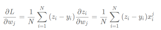
We can also use Numpy's mean function to do this:
# axis = 0 means add each row and divide by the total number of rows
gradient_w = np.mean(gradient_w, axis=0)
print('gradient_w ', gradient_w.shape)
print('w ', net.w.shape)
print(gradient_w)
print(net.w)
gradient_w  (13,)
w  (13, 1)
[ 1.59697064 -0.92928123  4.72726926  1.65712204  4.96176389  1.18068454
  4.55846519 -3.37770889  9.57465893 10.29870662  1.3900257  -0.30152215
  1.09276043]
[[ 1.76405235e+00]
 [ 4.00157208e-01]
 [ 9.78737984e-01]
 [ 2.24089320e+00]
 [ 1.86755799e+00]
 [ 1.59000000e+02]
 [ 9.50088418e-01]
 [-1.51357208e-01]
 [-1.03218852e-01]
 [ 1.59000000e+02]
 [ 1.44043571e-01]
 [ 1.45427351e+00]
 [ 7.61037725e-01]]
We use the matrix operation of numpy to complete the calculation of gradient conveniently, but we introduce a problem, gradient_ The shape of w is (13,), and the dimension of w is (13, 1). The cause of this problem is the use of np.mean The zero dimension is eliminated in function. For the convenience of addition, subtraction, multiplication and division, grade_ w and w must be in the same shape. So we will grade_ The dimension of w is also set to (13, 1), and the code is as follows:
gradient_w = gradient_w[:, np.newaxis]
print('gradient_w shape', gradient_w.shape)
gradient_w shape (13, 1)
In combination with the above discussion, the code to calculate the gradient is as follows.
z = net.forward(x)
gradient_w = (z - y) * x
gradient_w = np.mean(gradient_w, axis=0)
gradient_w = gradient_w[:, np.newaxis]
gradient_w
array([[ 1.59697064], [-0.92928123], [ 4.72726926], [ 1.65712204], [ 4.96176389], [ 1.18068454], [ 4.55846519], [-3.37770889], [ 9.57465893], [10.29870662], [ 1.3900257 ], [-0.30152215], [ 1.09276043]])
The above code is very concise to complete the gradient calculation of www. Similarly, the code that calculates the gradient of bbb is similar.
gradient_b = (z - y)
gradient_b = np.mean(gradient_b)
# Here b is a value, so you can directly use np.mean Get a scalar
gradient_b
-1.0918438870293816e-13
Write the above process of calculating the gradients of w and b as the gradientfunction of Network class, as shown below.
class Network(object):
    def __init__(self, num_of_weights):
        # Initial value of randomly generated w
        # In order to maintain the consistency of the results of each run of the program, a fixed random number seed is set here
        np.random.seed(0)
        self.w = np.random.randn(num_of_weights, 1)
        self.b = 0.

    def forward(self, x):
        z = np.dot(x, self.w) + self.b
        return z

    def loss(self, z, y):
        error = z - y
        num_samples = error.shape[0]
        cost = error * error
        cost = np.sum(cost) / num_samples
        return cost

    def gradient(self, x, y):
        z = self.forward(x)
        gradient_w = (z-y)*x
        gradient_w = np.mean(gradient_w, axis=0)
        gradient_w = gradient_w[:, np.newaxis]
        gradient_b = (z - y)
        gradient_b = np.mean(gradient_b)

        return gradient_w, gradient_b
# Call the gradient function defined above to calculate the gradient
# Initializing the network,
net = Network(13)
# Set [w5, w9] = [-100., +100.]
net.w[5] = -100.0
net.w[9] = -100.0

z = net.forward(x)
loss = net.loss(z, y)
gradient_w, gradient_b = net.gradient(x, y)
gradient_w5 = gradient_w[5][0]
gradient_w9 = gradient_w[9][0]
print('point {}, loss {}'.format([net.w[5][0], net.w[9][0]], loss))
print('gradient {}'.format([gradient_w5, gradient_w9]))
point [-100.0, -100.0], loss 686.3005008179159
gradient [-0.850073323995813, -6.138412364807849]
13: Identify points with smaller loss functions
Let's start to study the method of updating gradient. First, move a small step in the opposite direction of the gradient, find the next point P1, and observe the change of loss function.
# In the [w5, w9] plane, it moves to the next point P1 in the opposite direction of the gradient
# Define move step eta
eta = 0.1
# Update parameters w5 and w9
net.w[5] = net.w[5] - eta * gradient_w5
net.w[9] = net.w[9] - eta * gradient_w9
# Recalculate z and loss
z = net.forward(x)
loss = net.loss(z, y)
gradient_w, gradient_b = net.gradient(x, y)
gradient_w5 = gradient_w[5][0]
gradient_w9 = gradient_w[9][0]
print('point {}, loss {}'.format([net.w[5][0], net.w[9][0]], loss))
print('gradient {}'.format([gradient_w5, gradient_w9]))
point [-99.91499266760042, -99.38615876351922], loss 678.6472185028845
gradient [-0.8556356178645292, -6.0932268634065805]
Running the above code, you can find that taking a small step in the opposite direction of the gradient does reduce the loss function of the next point. If you are interested, you can try to click on the above code block to see if the loss function is getting smaller all the time.
In the above code, the statement used for each parameter update: net.w[5] = net.w[5] - eta * gradient_w5
- Subtraction: the parameter needs to move in the opposite direction of the gradient.
- eta: control the change of each parameter value along the reverse direction of the gradient, that is, the step length of each movement, also known as learning rate.
You can think about why we need to normalize the input characteristics and keep the scale consistent? This is to make the uniform step size more appropriate.
As shown in Figure 8, after the feature input is normalized, the Loss output of different parameters is a relatively regular curve, and the learning rate can be set to a unified value; when the feature input is not normalized, the steps required for the parameters corresponding to different features are not consistent, the parameters with larger scale need large steps, and the parameters with smaller size need small steps, which results in the inability to set a unified learning rate.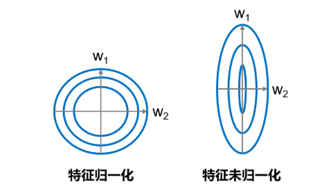
Figure 8: UN normalized features lead to different ideal steps for different feature dimensions
14: Code encapsulates the Train function
Encapsulate the calculation process of the above loop in the train and update functions, as shown below.
class Network(object):
def __init__(self, num_of_weights):
# Initial value of randomly generated w
# In order to maintain the consistency of the results of each run of the program, a fixed random number seed is set here
np.random.seed(0)
self.w = np.random.randn(num_of_weights,1)
self.w[5] = -100.
self.w[9] = -100.
self.b = 0.
def forward(self, x):
z = np.dot(x, self.w) + self.b
return z
def loss(self, z, y):
error = z - y
num_samples = error.shape[0]
cost = error * error
cost = np.sum(cost) / num_samples
return cost
def gradient(self, x, y):
z = self.forward(x)
gradient_w = (z-y)*x
gradient_w = np.mean(gradient_w, axis=0)
gradient_w = gradient_w[:, np.newaxis]
gradient_b = (z - y)
gradient_b = np.mean(gradient_b)
return gradient_w, gradient_b
def update(self, graident_w5, gradient_w9, eta=0.01):
net.w[5] = net.w[5] - eta * gradient_w5
net.w[9] = net.w[9] - eta * gradient_w9
def train(self, x, y, iterations=100, eta=0.01):
points = []
losses = []
for i in range(iterations):
points.append([net.w[5][0], net.w[9][0]])
z = self.forward(x)
L = self.loss(z, y)
gradient_w, gradient_b = self.gradient(x, y)
gradient_w5 = gradient_w[5][0]
gradient_w9 = gradient_w[9][0]
self.update(gradient_w5, gradient_w9, eta)
losses.append(L)
if i % 50 == 0:
print('iter {}, point {}, loss {}'.format(i, [net.w[5][0], net.w[9][0]], L))
return points, losses
# get data
train_data, test_data = load_data()
x = train_data[:, :-1]
y = train_data[:, -1:]
# Create a network
net = Network(13)
num_iterations=2000
# Start training
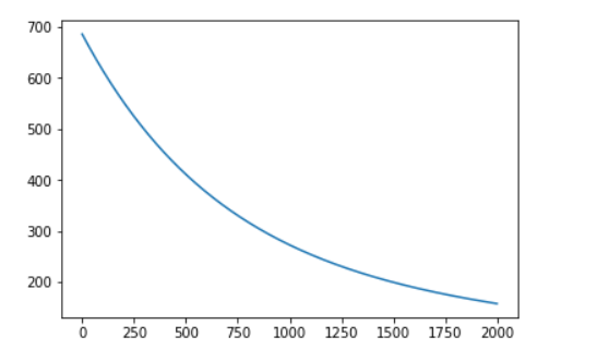
points, losses = net.train(x, y, iterations=num_iterations, eta=0.01)
# Draw the trend of loss function
plot_x = np.arange(num_iterations)
plot_y = np.array(losses)
plt.plot(plot_x, plot_y)
plt.show()
iter 0, point [-99.99144364382136, -99.93861587635192], loss 686.3005008179159
iter 50, point [-99.56362583488914, -96.92631128470325], loss 649.221346830939
iter 100, point [-99.13580802595692, -94.02279509580971], loss 614.6970095624063
iter 150, point [-98.7079902170247, -91.22404911807594], loss 582.543755023494
iter 200, point [-98.28017240809248, -88.52620357520894], loss 552.5911329872217
iter 250, point [-97.85235459916026, -85.9255316243737], loss 524.6810152322887
iter 300, point [-97.42453679022805, -83.41844407682491], loss 498.6667034691001
iter 350, point [-96.99671898129583, -81.00148431353688], loss 474.4121018974464
iter 400, point [-96.56890117236361, -78.67132338862874], loss 451.7909497114133
iter 450, point [-96.14108336343139, -76.42475531364933], loss 430.68610920670284
iter 500, point [-95.71326555449917, -74.25869251604028], loss 410.988905460488
iter 550, point [-95.28544774556696, -72.17016146534513], loss 392.5985138460824
iter 600, point [-94.85762993663474, -70.15629846096763], loss 375.4213919156372
iter 650, point [-94.42981212770252, -68.21434557551346], loss 359.3707524354014
iter 700, point [-94.0019943187703, -66.34164674796719], loss 344.36607459115214
iter 750, point [-93.57417650983808, -64.53564402117185], loss 330.33265059761464
iter 800, point [-93.14635870090586, -62.793873918279786], loss 317.2011651461846
iter 850, point [-92.71854089197365, -61.11396395304264], loss 304.907305311265
iter 900, point [-92.29072308304143, -59.49362926899678], loss 293.3913987080144
iter 950, point [-91.86290527410921, -57.930669402782904], loss 282.5980778542974
iter 1000, point [-91.43508746517699, -56.4229651670156], loss 272.47596883802515
iter 1050, point [-91.00726965624477, -54.968475648286564], loss 262.9774025287022
iter 1100, point [-90.57945184731255, -53.56523531604897], loss 254.05814669965383
iter 1150, point [-90.15163403838034, -52.21135123828792], loss 245.67715754581488
iter 1200, point [-89.72381622944812, -50.90500040003218], loss 237.796349191773
iter 1250, point [-89.2959984205159, -49.6444271209092], loss 230.3803798866218
iter 1300, point [-88.86818061158368, -48.42794056808474], loss 223.3964536766492
iter 1350, point [-88.44036280265146, -47.2539123610643], loss 216.81413643451378
iter 1400, point [-88.01254499371925, -46.12077426496303], loss 210.60518520483126
iter 1450, point [-87.58472718478703, -45.027015968976976], loss 204.74338990147896
iter 1500, point [-87.15690937585481, -43.9711829469081], loss 199.20442646183588
iter 1550, point [-86.72909156692259, -42.95187439671279], loss 193.96572062803054
iter 1600, point [-86.30127375799037, -41.96774125615467], loss 189.00632158541163
iter 1650, point [-85.87345594905815, -41.017484291751295], loss 184.3067847442463
iter 1700, point [-85.44563814012594, -40.0998522583068], loss 179.84906300239203
iter 1750, point [-85.01782033119372, -39.21364012642417], loss 175.61640587468244
iter 1800, point [-84.5900025222615, -38.35768737548557], loss 171.59326591927967
iter 1850, point [-84.16218471332928, -37.530876349682856], loss 167.76521193253296
iter 1900, point [-83.73436690439706, -36.73213067476985], loss 164.11884842217898
iter 1950, point [-83.30654909546485, -35.96041373329276], loss 160.64174090423475
class Network(object):
def __init__(self, num_of_weights):
# Initial value of randomly generated w
# In order to maintain the consistency of the results of each run of the program, a fixed random number seed is set here
np.random.seed(0)
self.w = np.random.randn(num_of_weights, 1)
self.b = 0.
def forward(self, x):
z = np.dot(x, self.w) + self.b
return z
def loss(self, z, y):
error = z - y
num_samples = error.shape[0]
cost = error * error
cost = np.sum(cost) / num_samples
return cost
def gradient(self, x, y):
z = self.forward(x)
gradient_w = (z-y)*x
gradient_w = np.mean(gradient_w, axis=0)
gradient_w = gradient_w[:, np.newaxis]
gradient_b = (z - y)
gradient_b = np.mean(gradient_b)
return gradient_w, gradient_b
def update(self, gradient_w, gradient_b, eta = 0.01):
self.w = self.w - eta * gradient_w
self.b = self.b - eta * gradient_b
def train(self, x, y, iterations=100, eta=0.01):
losses = []
for i in range(iterations):
z = self.forward(x)
L = self.loss(z, y)
gradient_w, gradient_b = self.gradient(x, y)
self.update(gradient_w, gradient_b, eta)
losses.append(L)
if (i+1) % 10 == 0:
print('iter {}, loss {}'.format(i, L))
return losses
# get data
train_data, test_data = load_data()
x = train_data[:, :-1]
y = train_data[:, -1:]
# Create a network
net = Network(13)
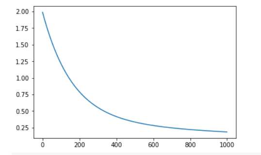
num_iterations=1000
# Start training
losses = net.train(x,y, iterations=num_iterations, eta=0.01)
# Draw the trend of loss function
plot_x = np.arange(num_iterations)
plot_y = np.array(losses)
plt.plot(plot_x, plot_y)
plt.show()
iter 9, loss 1.8984947314576224
iter 19, loss 1.8031783384598725
iter 29, loss 1.7135517565541092
iter 39, loss 1.6292649416831264
iter 49, loss 1.5499895293373231
iter 59, loss 1.4754174896452612
iter 69, loss 1.4052598659324693
iter 79, loss 1.3392455915676864
iter 89, loss 1.2771203802372915
iter 99, loss 1.218645685090292
iter 109, loss 1.1635977224791534
iter 119, loss 1.111766556287068
iter 129, loss 1.0629552390811503
iter 139, loss 1.0169790065644477
iter 149, loss 0.9736645220185994
iter 159, loss 0.9328491676343147
iter 169, loss 0.8943803798194307
iter 179, loss 0.8581150257549611
iter 189, loss 0.8239188186389669
iter 199, loss 0.7916657692169988
iter 209, loss 0.761237671346902
iter 219, loss 0.7325236194855752
iter 229, loss 0.7054195561163928
iter 239, loss 0.6798278472589763
iter 249, loss 0.6556568843183528
iter 259, loss 0.6328207106387195
iter 269, loss 0.6112386712285092
iter 279, loss 0.59083508421862
iter 289, loss 0.5715389327049418
iter 299, loss 0.5532835757100347
iter 309, loss 0.5360064770773406
iter 319, loss 0.5196489511849665
iter 329, loss 0.5041559244351539
iter 339, loss 0.48947571154034963
iter 349, loss 0.47555980568755696
iter 359, loss 0.46236268171965056
iter 369, loss 0.44984161152579916
iter 379, loss 0.43795649088328303
iter 389, loss 0.4266696770400226
iter 399, loss 0.41594583637124666
iter 409, loss 0.4057518014851036
iter 419, loss 0.3960564371908221
iter 429, loss 0.38683051477942226
iter 439, loss 0.3780465941011246
iter 449, loss 0.3696789129556087
iter 459, loss 0.3617032833413179
iter 469, loss 0.3540969941381648
iter 479, loss 0.3468387198244131
iter 489, loss 0.3399084348532937
iter 499, loss 0.33328733333814486
iter 509, loss 0.3269577537166779
iter 519, loss 0.32090310808539985
iter 529, loss 0.3151078159144129
iter 539, loss 0.30955724187078903
iter 549, loss 0.3042376374955925
iter 559, loss 0.2991360864954391
iter 569, loss 0.2942404534243286
iter 579, loss 0.2895393355454012
iter 589, loss 0.28502201767532415
iter 599, loss 0.28067842982626157
iter 609, loss 0.27649910747186535
iter 619, loss 0.2724751542744919
iter 629, loss 0.2685982071209627
iter 639, loss 0.26486040332365085
iter 649, loss 0.2612543498525749
iter 659, loss 0.2577730944725093
iter 669, loss 0.2544100986669443
iter 679, loss 0.2511592122380609
iter 689, loss 0.2480146494787638
iter 699, loss 0.24497096681926708
iter 709, loss 0.2420230418567802
iter 719, loss 0.23916605368251415
iter 729, loss 0.23639546442555454
iter 739, loss 0.23370700193813704
iter 749, loss 0.2310966435515475
iter 759, loss 0.2285606008362593
iter 769, loss 0.22609530530403904
iter 779, loss 0.22369739499361888
iter 789, loss 0.2213637018851542
iter 799, loss 0.21909124009208833
iter 809, loss 0.21687719478222933
iter 819, loss 0.21471891178284025
iter 829, loss 0.21261388782734392
iter 839, loss 0.2105597614038757
iter 849, loss 0.20855430416838638
iter 859, loss 0.20659541288730932
iter 869, loss 0.20468110187697833
iter 879, loss 0.2028094959090178
iter 889, loss 0.20097882355283644
iter 899, loss 0.19918741092814596
iter 909, loss 0.19743367584210875
iter 919, loss 0.1957161222872899
iter 929, loss 0.19403333527807176
iter 939, loss 0.19238397600456975
iter 949, loss 0.19076677728439412
iter 959, loss 0.1891805392938162
iter 969, loss 0.18762412556104593
iter 979, loss 0.18609645920539716
iter 989, loss 0.18459651940712488
iter 999, loss 0.18312333809366155
15: Stochastic Gradient Descent
In the above program, each loss function and gradient calculation is based on the total data in the data set. For the Boston house price forecasting task data set, the sample number is relatively small, only 404. However, in practical problems, data sets are often very large. If full data is used for calculation every time, the efficiency is very low. Generally speaking, it is "killing chickens without using ox knives". Since the parameters only update a little bit in the opposite direction of the gradient at a time, the direction does not need to be so precise. A reasonable solution is to randomly extract a small part of data from the total data set each time to represent the whole. Based on this part of data, calculate the gradient and loss to update the parameters. This method is called the Stochastic Gradient Descent (SGD). The core concepts are as follows:
- Min batch: a batch of data extracted at each iteration is called a min batch.
- batch_size: the number of samples contained in a mini batch is called batch_size.
- Epoch: when the program iterates, the samples are gradually extracted according to mini batch. When the entire data set is traversed, a round of training, also called an epoch, is completed. When starting training, you can num the number of training rounds_ Epochs and batch_size is passed in as a parameter.
The following describes the specific implementation process with the program, involving data processing and training process two parts of the code modification.
16: Data processing code modification
Data processing needs two functions: splitting data batches and disordering samples (in order to achieve the effect of random sampling).
# get data
train_data, test_data = load_data()
train_data.shape
(404, 14)
train_data contains 404 pieces of data in total. If batch_size=10, i.e. take the first 0-9 sample as the first mini batch, and name the train_data1.
train_data1 = train_data[0:10]
train_data1.shape
(10, 14)
Using train_ The data of data1 (sample 0-9) calculates the gradient and updates the network parameters.
net = Network(13)
x = train_data1[:, :-1]
y = train_data1[:, -1:]
loss = net.train(x, y, iterations=1, eta=0.01)
loss
[0.9001866101467375]
Then take sample 10-19 as the second Mini batch, calculate the gradient and update the network parameters.
train_data2 = train_data[10:19]
x = train_data1[:, :-1]
y = train_data1[:, -1:]
loss = net.train(x, y, iterations=1, eta=0.01)
loss
[0.8903272433979657]
According to this method, new mini batch is taken out and network parameters are updated gradually.
Next, we will train_data is divided into batch size_ Multiple mini of size_ Batch, as shown in the following code: set the train_data is divided into 104 / 40 + 1 = 41 mini_batch, the top 40 mini_batch, each containing 10 samples and the last mini_batch contains only four samples.
batch_size = 10
n = len(train_data)
mini_batches = [train_data[k:k+batch_size] for k in range(0, n, batch_size)]
print('total number of mini_batches is ', len(mini_batches))
print('first mini_batch shape ', mini_batches[0].shape)
print('last mini_batch shape ', mini_batches[-1].shape)
total number of mini_batches is  41
first mini_batch shape  (10, 14)
last mini_batch shape  (4, 14)
In addition, we take out Mini in order_ Batch, and SGD is a random sampling part of the sample to represent the population. In order to achieve the effect of random sampling, we first put the train_ The sample order in data is randomly scrambled, and then Mini is extracted_ batch. Randomly disorder the sample order, which needs to be used np.random.shuffle Function, its usage will be introduced first.
explain:
Through a large number of experiments, it is found that the model is more impressed by the final data. After the training data is imported, the closer to the end of the model training, the greater the impact of the last batch data on the model parameters. In order to avoid the influence of model memory on training effect, it is necessary to carry out the operation of sample disorder.
# Create a new array
a = np.array([1,2,3,4,5,6,7,8,9,10,11,12])
print('before shuffle', a)
np.random.shuffle(a)
print('after shuffle', a)
before shuffle [ 1  2  3  4  5  6  7  8  9 10 11 12]
after shuffle [ 7  2 11  3  8  6 12  1  4  5 10  9]
Running the above code several times, you can find that the number order is different after each shuffle function execution. The above is a case of 1-dimensional array disorder. We observe the effect of 2-dimensional array disorder.
# Create a new array
a = np.array([1,2,3,4,5,6,7,8,9,10,11,12])
a = a.reshape([6, 2])
print('before shuffle\n', a)
np.random.shuffle(a)
print('after shuffle\n', a)
before shuffle
 [[ 1  2]
 [ 3  4]
 [ 5  6]
 [ 7  8]
 [ 9 10]
 [11 12]]
after shuffle
 [[ 1  2]
 [ 3  4]
 [ 5  6]
 [ 9 10]
 [11 12]
 [ 7  8]]
It is found that the elements of the array are randomly scrambled in dimension 0, but the order of dimension 1 remains unchanged. For example, the number 2 is still next to the number 1, the number 8 is still next to the number 7, and the [3,4] of the second dimension is not next to the [1,2]. Integrate this part of the SGD algorithm code into the train function in the Network class, and the final complete code is as follows.
# get data
train_data, test_data = load_data()

# Scramble sample order
np.random.shuffle(train_data)

# train_data is divided into multiple mini_batch
batch_size = 10
n = len(train_data)
mini_batches = [train_data[k:k+batch_size] for k in range(0, n, batch_size)]

# Create a network
net = Network(13)

# Use each mini in turn_ Batch data
for mini_batch in mini_batches:
    x = mini_batch[:, :-1]
    y = mini_batch[:, -1:]
    loss = net.train(x, y, iterations=1)
17: Training process code modification
Each randomly selected Mini batch data is input into the model for parameter training. The core of the training process is two levels of circulation:
1: The first level loop, which represents the sample set to be trained to traverse several times, is called "epoch". The code is as follows:
for epoch_id in range(num_epoches):
2: The second layer is a loop, which represents the multiple batches that the sample set is split into each time it is traversed. All the training needs to be performed, which is called "iter (iteration)",
The code is as follows: for iter_id,mini_batch in emumerate(mini_batches):
Inside the two-level cycle is the classic four-step training process: forward calculation - > calculation loss - > calculation gradient - > update parameters, which is consistent with what you have learned before. The code is as follows:
        x = mini_batch[:, :-1]
        y = mini_batch[:, -1:]
        a = self.forward(x)  #Forward calculation
        loss = self.loss(a, y)  #Calculate loss
        gradient_w, gradient_b = self.gradient(x, y)  #Calculation gradient
        self.update(gradient_w, gradient_b, eta)  #Update parameters
The final implementation is as follows.
import numpy as np
class Network(object):
def __init__(self, num_of_weights):
# Initial value of randomly generated w
# In order to maintain the consistency of the results of each run of the program, a fixed random number seed is set here
#np.random.seed(0)
self.w = np.random.randn(num_of_weights, 1)
self.b = 0.
def forward(self, x):
z = np.dot(x, self.w) + self.b
return z
def loss(self, z, y):
error = z - y
num_samples = error.shape[0]
cost = error * error
cost = np.sum(cost) / num_samples
return cost
def gradient(self, x, y):
z = self.forward(x)
N = x.shape[0]
gradient_w = 1. / N * np.sum((z-y) * x, axis=0)
gradient_w = gradient_w[:, np.newaxis]
gradient_b = 1. / N * np.sum(z-y)
return gradient_w, gradient_b
def update(self, gradient_w, gradient_b, eta = 0.01):
self.w = self.w - eta * gradient_w
self.b = self.b - eta * gradient_b
def train(self, training_data, num_epoches, batch_size=10, eta=0.01):
n = len(training_data)
losses = []
for epoch_id in range(num_epoches):
# Before each iteration, the order of training data is randomly disrupted,
# And then press batch every time_ How to retrieve size data
np.random.shuffle(training_data)
# Split the training data, each mini_batch contains batch_ Data of size bar
mini_batches = [training_data[k:k+batch_size] for k in range(0, n, batch_size)]
for iter_id, mini_batch in enumerate(mini_batches):
#print(self.w.shape)
#print(self.b)
x = mini_batch[:, :-1]
y = mini_batch[:, -1:]
a = self.forward(x)
loss = self.loss(a, y)
gradient_w, gradient_b = self.gradient(x, y)
self.update(gradient_w, gradient_b, eta)
losses.append(loss)
print('Epoch {:3d} / iter {:3d}, loss = {:.4f}'.
format(epoch_id, iter_id, loss))
return losses
# get data
train_data, test_data = load_data()
# Create a network
net = Network(13)
# Start training
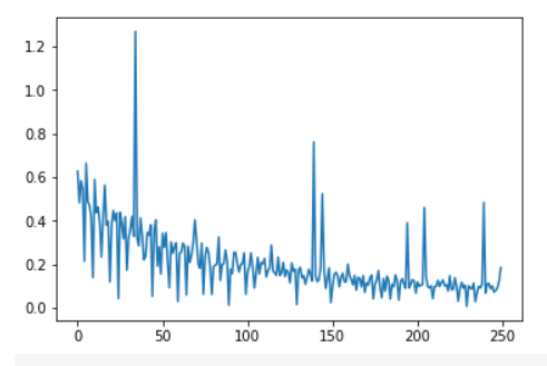
losses = net.train(train_data, num_epoches=50, batch_size=100, eta=0.1)
# Draw the trend of loss function
plot_x = np.arange(len(losses))
plot_y = np.array(losses)
plt.plot(plot_x, plot_y)
plt.show()
Epoch 0 / iter 0, loss = 0.6273
Epoch 0 / iter 1, loss = 0.4835
Epoch 0 / iter 2, loss = 0.5830
Epoch 0 / iter 3, loss = 0.5466
Epoch 0 / iter 4, loss = 0.2147
Epoch 1 / iter 0, loss = 0.6645
Epoch 1 / iter 1, loss = 0.4875
Epoch 1 / iter 2, loss = 0.4707
Epoch 1 / iter 3, loss = 0.4153
Epoch 1 / iter 4, loss = 0.1402
Epoch 2 / iter 0, loss = 0.5897
Epoch 2 / iter 1, loss = 0.4373
Epoch 2 / iter 2, loss = 0.4631
Epoch 2 / iter 3, loss = 0.3960
Epoch 2 / iter 4, loss = 0.2340
Epoch 3 / iter 0, loss = 0.4139
Epoch 3 / iter 1, loss = 0.5635
Epoch 3 / iter 2, loss = 0.3807
Epoch 3 / iter 3, loss = 0.3975
Epoch 3 / iter 4, loss = 0.1207
Epoch 4 / iter 0, loss = 0.3786
Epoch 4 / iter 1, loss = 0.4474
Epoch 4 / iter 2, loss = 0.4019
Epoch 4 / iter 3, loss = 0.4352
Epoch 4 / iter 4, loss = 0.0435
Epoch 5 / iter 0, loss = 0.4387
Epoch 5 / iter 1, loss = 0.3886
Epoch 5 / iter 2, loss = 0.3182
Epoch 5 / iter 3, loss = 0.4189
Epoch 5 / iter 4, loss = 0.1741
Epoch 6 / iter 0, loss = 0.3191
Epoch 6 / iter 1, loss = 0.3601
Epoch 6 / iter 2, loss = 0.4199
Epoch 6 / iter 3, loss = 0.3289
Epoch 6 / iter 4, loss = 1.2691
Epoch 7 / iter 0, loss = 0.3202
Epoch 7 / iter 1, loss = 0.2855
Epoch 7 / iter 2, loss = 0.4129
Epoch 7 / iter 3, loss = 0.3331
Epoch 7 / iter 4, loss = 0.2218
Epoch 8 / iter 0, loss = 0.2368
Epoch 8 / iter 1, loss = 0.3457
Epoch 8 / iter 2, loss = 0.3339
Epoch 8 / iter 3, loss = 0.3812
Epoch 8 / iter 4, loss = 0.0534
Epoch 9 / iter 0, loss = 0.3567
Epoch 9 / iter 1, loss = 0.4033
Epoch 9 / iter 2, loss = 0.1926
Epoch 9 / iter 3, loss = 0.2803
Epoch 9 / iter 4, loss = 0.1557
Epoch 10 / iter 0, loss = 0.3435
Epoch 10 / iter 1, loss = 0.2790
Epoch 10 / iter 2, loss = 0.3456
Epoch 10 / iter 3, loss = 0.2076
Epoch 10 / iter 4, loss = 0.0935
Epoch 11 / iter 0, loss = 0.3024
Epoch 11 / iter 1, loss = 0.2517
Epoch 11 / iter 2, loss = 0.2797
Epoch 11 / iter 3, loss = 0.2989
Epoch 11 / iter 4, loss = 0.0301
Epoch 12 / iter 0, loss = 0.2507
Epoch 12 / iter 1, loss = 0.2563
Epoch 12 / iter 2, loss = 0.2971
Epoch 12 / iter 3, loss = 0.2833
Epoch 12 / iter 4, loss = 0.0597
Epoch 13 / iter 0, loss = 0.2827
Epoch 13 / iter 1, loss = 0.2094
Epoch 13 / iter 2, loss = 0.2417
Epoch 13 / iter 3, loss = 0.2985
Epoch 13 / iter 4, loss = 0.4036
Epoch 14 / iter 0, loss = 0.3085
Epoch 14 / iter 1, loss = 0.2015
Epoch 14 / iter 2, loss = 0.1830
Epoch 14 / iter 3, loss = 0.2978
Epoch 14 / iter 4, loss = 0.0630
Epoch 15 / iter 0, loss = 0.2342
Epoch 15 / iter 1, loss = 0.2780
Epoch 15 / iter 2, loss = 0.2571
Epoch 15 / iter 3, loss = 0.1838
Epoch 15 / iter 4, loss = 0.0627
Epoch 16 / iter 0, loss = 0.1896
Epoch 16 / iter 1, loss = 0.1966
Epoch 16 / iter 2, loss = 0.2018
Epoch 16 / iter 3, loss = 0.3257
Epoch 16 / iter 4, loss = 0.1268
Epoch 17 / iter 0, loss = 0.1990
Epoch 17 / iter 1, loss = 0.2031
Epoch 17 / iter 2, loss = 0.2662
Epoch 17 / iter 3, loss = 0.2128
Epoch 17 / iter 4, loss = 0.0133
Epoch 18 / iter 0, loss = 0.1780
Epoch 18 / iter 1, loss = 0.1575
Epoch 18 / iter 2, loss = 0.2547
Epoch 18 / iter 3, loss = 0.2544
Epoch 18 / iter 4, loss = 0.2007
Epoch 19 / iter 0, loss = 0.1657
Epoch 19 / iter 1, loss = 0.2000
Epoch 19 / iter 2, loss = 0.2045
Epoch 19 / iter 3, loss = 0.2524
Epoch 19 / iter 4, loss = 0.0632
Epoch 20 / iter 0, loss = 0.1629
Epoch 20 / iter 1, loss = 0.1895
Epoch 20 / iter 2, loss = 0.2523
Epoch 20 / iter 3, loss = 0.1896
Epoch 20 / iter 4, loss = 0.0918
Epoch 21 / iter 0, loss = 0.1583
Epoch 21 / iter 1, loss = 0.2322
Epoch 21 / iter 2, loss = 0.1567
Epoch 21 / iter 3, loss = 0.2089
Epoch 21 / iter 4, loss = 0.2035
Epoch 22 / iter 0, loss = 0.2273
Epoch 22 / iter 1, loss = 0.1427
Epoch 22 / iter 2, loss = 0.1712
Epoch 22 / iter 3, loss = 0.1826
Epoch 22 / iter 4, loss = 0.2878
Epoch 23 / iter 0, loss = 0.1685
Epoch 23 / iter 1, loss = 0.1622
Epoch 23 / iter 2, loss = 0.1499
Epoch 23 / iter 3, loss = 0.2329
Epoch 23 / iter 4, loss = 0.1486
Epoch 24 / iter 0, loss = 0.1617
Epoch 24 / iter 1, loss = 0.2083
Epoch 24 / iter 2, loss = 0.1442
Epoch 24 / iter 3, loss = 0.1740
Epoch 24 / iter 4, loss = 0.1641
Epoch 25 / iter 0, loss = 0.1159
Epoch 25 / iter 1, loss = 0.2064
Epoch 25 / iter 2, loss = 0.1690
Epoch 25 / iter 3, loss = 0.1778
Epoch 25 / iter 4, loss = 0.0159
Epoch 26 / iter 0, loss = 0.1730
Epoch 26 / iter 1, loss = 0.1861
Epoch 26 / iter 2, loss = 0.1387
Epoch 26 / iter 3, loss = 0.1486
Epoch 26 / iter 4, loss = 0.1090
Epoch 27 / iter 0, loss = 0.1393
Epoch 27 / iter 1, loss = 0.1775
Epoch 27 / iter 2, loss = 0.1564
Epoch 27 / iter 3, loss = 0.1245
Epoch 27 / iter 4, loss = 0.7611
Epoch 28 / iter 0, loss = 0.1470
Epoch 28 / iter 1, loss = 0.1211
Epoch 28 / iter 2, loss = 0.1285
Epoch 28 / iter 3, loss = 0.1854
Epoch 28 / iter 4, loss = 0.5240
Epoch 29 / iter 0, loss = 0.1740
Epoch 29 / iter 1, loss = 0.0898
Epoch 29 / iter 2, loss = 0.1392
Epoch 29 / iter 3, loss = 0.1842
Epoch 29 / iter 4, loss = 0.0251
Epoch 30 / iter 0, loss = 0.0978
Epoch 30 / iter 1, loss = 0.1529
Epoch 30 / iter 2, loss = 0.1640
Epoch 30 / iter 3, loss = 0.1503
Epoch 30 / iter 4, loss = 0.0975
Epoch 31 / iter 0, loss = 0.1399
Epoch 31 / iter 1, loss = 0.1595
Epoch 31 / iter 2, loss = 0.1209
Epoch 31 / iter 3, loss = 0.1203
Epoch 31 / iter 4, loss = 0.2008
Epoch 32 / iter 0, loss = 0.1501
Epoch 32 / iter 1, loss = 0.1310
Epoch 32 / iter 2, loss = 0.1065
Epoch 32 / iter 3, loss = 0.1489
Epoch 32 / iter 4, loss = 0.0818
Epoch 33 / iter 0, loss = 0.1401
Epoch 33 / iter 1, loss = 0.1367
Epoch 33 / iter 2, loss = 0.0970
Epoch 33 / iter 3, loss = 0.1481
Epoch 33 / iter 4, loss = 0.0711
Epoch 34 / iter 0, loss = 0.1157
Epoch 34 / iter 1, loss = 0.1050
Epoch 34 / iter 2, loss = 0.1378
Epoch 34 / iter 3, loss = 0.1505
Epoch 34 / iter 4, loss = 0.0429
Epoch 35 / iter 0, loss = 0.1096
Epoch 35 / iter 1, loss = 0.1279
Epoch 35 / iter 2, loss = 0.1715
Epoch 35 / iter 3, loss = 0.0888
Epoch 35 / iter 4, loss = 0.0473
Epoch 36 / iter 0, loss = 0.1350
Epoch 36 / iter 1, loss = 0.0781
Epoch 36 / iter 2, loss = 0.1458
Epoch 36 / iter 3, loss = 0.1288
Epoch 36 / iter 4, loss = 0.0421
Epoch 37 / iter 0, loss = 0.1083
Epoch 37 / iter 1, loss = 0.0972
Epoch 37 / iter 2, loss = 0.1513
Epoch 37 / iter 3, loss = 0.1236
Epoch 37 / iter 4, loss = 0.0366
Epoch 38 / iter 0, loss = 0.1204
Epoch 38 / iter 1, loss = 0.1341
Epoch 38 / iter 2, loss = 0.1109
Epoch 38 / iter 3, loss = 0.0905
Epoch 38 / iter 4, loss = 0.3906
Epoch 39 / iter 0, loss = 0.0923
Epoch 39 / iter 1, loss = 0.1094
Epoch 39 / iter 2, loss = 0.1295
Epoch 39 / iter 3, loss = 0.1239
Epoch 39 / iter 4, loss = 0.0684
Epoch 40 / iter 0, loss = 0.1188
Epoch 40 / iter 1, loss = 0.0984
Epoch 40 / iter 2, loss = 0.1067
Epoch 40 / iter 3, loss = 0.1057
Epoch 40 / iter 4, loss = 0.4602
Epoch 41 / iter 0, loss = 0.1478
Epoch 41 / iter 1, loss = 0.0980
Epoch 41 / iter 2, loss = 0.0921
Epoch 41 / iter 3, loss = 0.1020
Epoch 41 / iter 4, loss = 0.0430
Epoch 42 / iter 0, loss = 0.0991
Epoch 42 / iter 1, loss = 0.0994
Epoch 42 / iter 2, loss = 0.1270
Epoch 42 / iter 3, loss = 0.0988
Epoch 42 / iter 4, loss = 0.1176
Epoch 43 / iter 0, loss = 0.1286
Epoch 43 / iter 1, loss = 0.1013
Epoch 43 / iter 2, loss = 0.1066
Epoch 43 / iter 3, loss = 0.0779
Epoch 43 / iter 4, loss = 0.1481
Epoch 44 / iter 0, loss = 0.0840
Epoch 44 / iter 1, loss = 0.0858
Epoch 44 / iter 2, loss = 0.1388
Epoch 44 / iter 3, loss = 0.1000
Epoch 44 / iter 4, loss = 0.0313
Epoch 45 / iter 0, loss = 0.0896
Epoch 45 / iter 1, loss = 0.1173
Epoch 45 / iter 2, loss = 0.0916
Epoch 45 / iter 3, loss = 0.1043
Epoch 45 / iter 4, loss = 0.0074
Epoch 46 / iter 0, loss = 0.1008
Epoch 46 / iter 1, loss = 0.0915
Epoch 46 / iter 2, loss = 0.0877
Epoch 46 / iter 3, loss = 0.1139
Epoch 46 / iter 4, loss = 0.0292
Epoch 47 / iter 0, loss = 0.0679
Epoch 47 / iter 1, loss = 0.0987
Epoch 47 / iter 2, loss = 0.0929
Epoch 47 / iter 3, loss = 0.1098
Epoch 47 / iter 4, loss = 0.4838
Epoch 48 / iter 0, loss = 0.0693
Epoch 48 / iter 1, loss = 0.1095
Epoch 48 / iter 2, loss = 0.1128
Epoch 48 / iter 3, loss = 0.0890
Epoch 48 / iter 4, loss = 0.1008
Epoch 49 / iter 0, loss = 0.0724
Epoch 49 / iter 1, loss = 0.0804
Epoch 49 / iter 2, loss = 0.0919
Epoch 49 / iter 3, loss = 0.1233
Epoch 49 / iter 4, loss = 0.1849
explain:
Because the data volume of house price prediction is too small, it is difficult to feel the performance improvement brought by random gradient decline.
summary
In this section, we explained in detail how to use Numpy to realize the gradient descent algorithm, and constructed and trained a simple linear model to realize the Boston house price prediction. We can conclude that there are three main points to use neural network to model the house price prediction:
- Construct the network, initialize the parameters w and b, and define the calculation method of prediction and loss function.
- The initial point is selected randomly, and the gradient calculation method and parameter updating method are established.
- Extract part of the data from the total data set as a mini_batch, calculate the gradient and update the parameters, and continue to iterate until the loss function almost no longer drops.
Basic knowledge
- The chain rule of derivation
The chain rule is the derivative rule in calculus, which is used to find the derivative of a compound function. It is a common method in the derivative operation of calculus. The derivative of a composite function is the product of the derivative of the finite composite function at the corresponding point, just like a chain, which is called the chain rule. As shown in Figure 9, if the gradient of the final output to the inner input (the first layer) is calculated, it is equal to the gradient of the outer gradient (the second layer) multiplied by the gradient of the function of this layer.
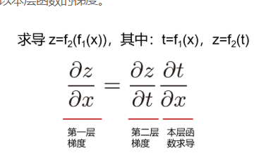
Figure 9: chain rule of derivation
- The concept of calculation graph
(1) Why reverse gradient? That is, the gradient is calculated from the back-end to the front-end of the network. The gradient of the current layer should be calculated according to the gradient of the next layer in the network, so only the gradient of the next layer can be calculated.
(2) Case: calculation chart of consumption generated by purchasing apple. Let's say a store sells apple at a discount of 10%, and the unit price of each is 100 yuan. The structure of calculating a customer's total consumption is shown in Figure 10.
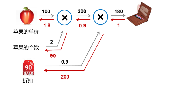
Figure 10: consumption calculation chart of Apple purchase
- Forward calculation process: indicated by the black arrow, the customer bought 2 apples, plus a 10% discount, and the total consumption was 10020.9 = 180 yuan.
- Backward propagation process: indicated by the red arrow, according to the chain rule, the gradient of this layer is calculated * the gradient transferred from the next layer, so it needs to be calculated from the back to the front.
The output of the last layer differentiates itself to 1. The second derivative layer is 0.91 and 2001 respectively according to the formula of multiplication and derivation shown in FIG. 11. Similarly, the third layer is 100 * 0.9 = 90, and 2 * 0.9 = 1.8.
Figure 11: formula for multiplication and derivation