Impulse neural network is called the third generation neural network, which has higher biological reliability. SNN has always occupied the core position in the research of brain like science in recent years. When the performance is similar, the chip based on pulse neural network has lower power consumption, better stability and robustness than artificial neural network.
Brian2 is installed through pip, and some programs provided on the official website are run. Some learning experiences are also attached.

from brian2 import *
start_scope()
#start_ The scope () function ensures that any changes created before the function is called 
#Brian objects will not be included in the next simulation run.
tau = 10*ms
eqs ='dv/dt = (1-v)/tau : 1'
G = NeuronGroup(1, eqs,method='exact')
print('Before v = %s' % G.v[0])
run(100*ms)
print('After v = %s' % G.v[0])
start_scope()
G = NeuronGroup(1, eqs, method='exact')
M = StateMonitor(G, 'v', record=0)
run(30*ms)
plot(M.t/ms, M.v[0], 'C0', label='Brian')
plot(M.t/ms, 1-exp(-M.t/tau), 'C1--',label='Analytic')
xlabel('Time (ms)')
ylabel('v')
legend()
show()

Pay attention to dimensions in the program. If the quantities of different units are added, and the dimensions on the left and right of the equation are inconsistent, the program will report errors. If / tau is removed from EQS = 'DV / dt = (1-V) / tau: 1', an error will be reported due to dimensional inconsistency.

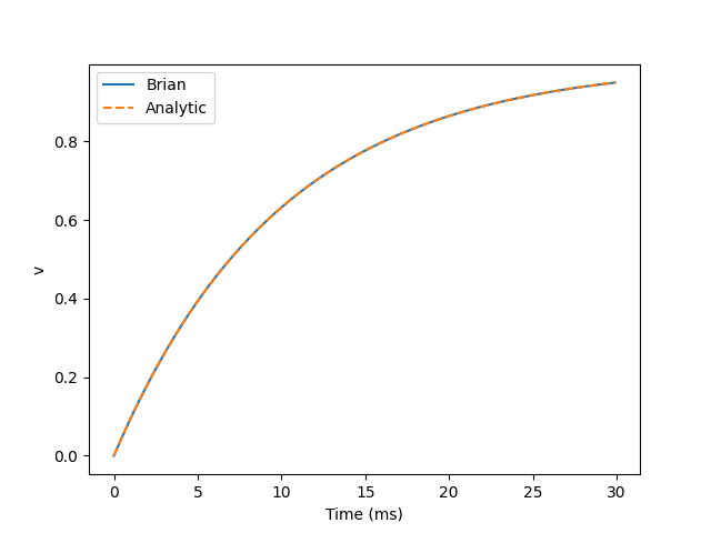
In this program, the neuron group function NeuronGroup () creates a neuron with a model defined by the differential equation DV / dt = (1-V) / tau: 1. We use the StateMonitor function to monitor the neuron state. The first two parameters are the group to be recorded and the variable to be recorded. We also specify record=0. This means that we record all values of neuron 0. We must specify which neurons we want to record, because in a large simulation with many neurons, it usually takes up too much RAM to record the values of all neurons.

The blue solid line is the change of the neuron v, and the orange dotted line is the function curve of the analytical solution 1-exp(-t/tau) of the differential equation DV / dt = (1-v) / tau: 1. The two coincide.

start_scope()
tau = 10*ms
eqs = '''
dv/dt = (1-v)/tau : 1
'''
G = NeuronGroup(1, eqs, threshold='v>0.8', reset='v = 0', method='exact')
M = StateMonitor(G, 'v', record=0)
run(50*ms)
plot(M.t/ms, M.v[0])
xlabel('Time (ms)')
ylabel('v')
show()

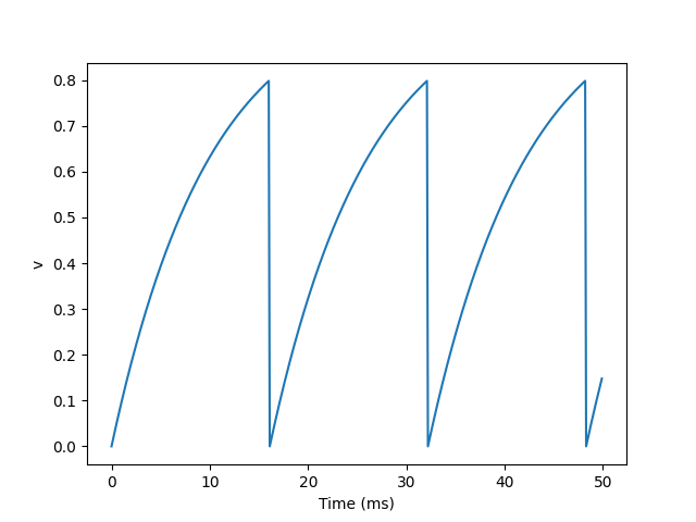
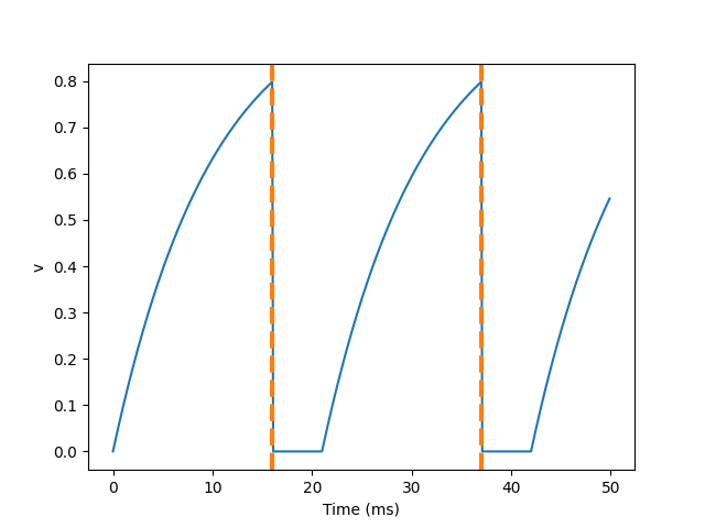
We added two new keywords to the neurogroup declaration: threshold ='v > 0.8 'and reset='v = 0'. This means that when we launch a spike, we reset it immediately after the spike.

from brian2 import *
start_scope()
tau = 10*ms
eqs ='dv/dt = (1-v)/tau : 1'
G = NeuronGroup(1, eqs, threshold='v>0.8', reset='v = 0', method='exact')
statemon = StateMonitor(G, 'v', record=0)
spikemon = SpikeMonitor(G)
run(50*ms)
print('Spike times: %s' % spikemon.t[:])
plot(statemon.t/ms, statemon.v[0])
for t in spikemon.t:
    axvline(t/ms, ls='--', c='C1', lw=3)
xlabel('Time (ms)')
ylabel('v')
show()

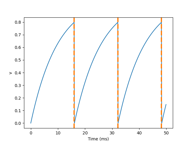
Pulse times: [16. 32.1 48.2] MS

A common feature of neuronal models is refractory period. This means that after a neuron emits a spike, it becomes stubborn for a period of time, and can't launch another spike until the end of this period. Here's what we did in Brian.

from brian2 import *
start_scope()
tau = 10*ms
eqs ='dv/dt = (1-v)/tau : 1'
start_scope()
tau = 10*ms
eqs = '''
dv/dt = (1-v)/tau : 1 (unless refractory)
'''
G = NeuronGroup(1, eqs, threshold='v>0.8', reset='v = 0', refractory=5*ms, method='exact')
statemon = StateMonitor(G, 'v', record=0)
spikemon = SpikeMonitor(G)
run(50*ms)
plot(statemon.t/ms, statemon.v[0])
for t in spikemon.t:
    axvline(t/ms, ls='--', c='C1', lw=3)
xlabel('Time (ms)')
ylabel('v')
show()

Although we added the parameter refactory = 5 * MS to the neurogroup function, we still need to add (unless refactory) to the differential equation, otherwise the behavior of neurons will not produce refractory period.

from brian2 import *
start_scope()
tau = 5*ms
eqs = '''
dv/dt = (1-v)/tau : 1
'''
G = NeuronGroup(1, eqs, threshold='v>0.8', reset='v = 0', refractory=15*ms, method='exact')
statemon = StateMonitor(G, 'v', record=0)
spikemon = SpikeMonitor(G)
run(50*ms)
plot(statemon.t/ms, statemon.v[0])
for t in spikemon.t:
    axvline(t/ms, ls='--', c='C1', lw=3)
axhline(0.8, ls=':', c='C2', lw=3)
xlabel('Time (ms)')
ylabel('v')
print("Spike times: %s" % spikemon.t[:])
show()

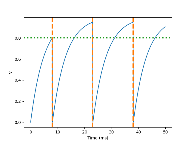
So what happened here? The behavior of the first spike is the same: v rises to 0.8, then the neuron triggers the spike in 0 to 8 milliseconds, and then resets to 0 immediately. Since the refractory period is now 15 ms, this means that neurons will not spike again until time 8 + 15 = 23 Ms. After the first peak, the value of v starts to rise immediately, because we do not specify (unless reflex) in the definition of neurogroup. At this time, although it can reach the value of 0.8 (green dotted line) in about 8 milliseconds, because the neuron is now in refractory period, it will not reset but continue to rise after reaching the threshold, The potential will not be reset until the end of the refractory period.

Multiple neurons are shown below.

from brian2 import *
start_scope()
N = 100
tau = 10*ms
eqs = '''
dv/dt = (2-v)/tau : 1
'''
G = NeuronGroup(N, eqs, threshold='v>1', reset='v=0', method='exact')
G.v = 'rand()'
spikemon = SpikeMonitor(G)
run(50*ms)
plot(spikemon.t/ms, spikemon.i, '.k')
xlabel('Time (ms)')
ylabel('Neuron index')
show()

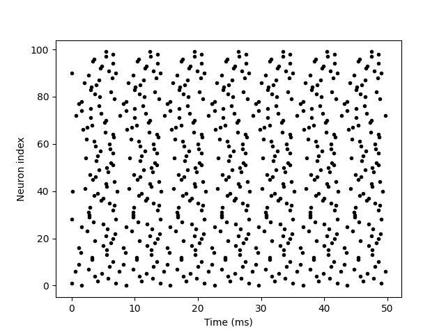
Variable N is used to determine the number of neurons. G.v = 'rand()' initializes each neuron with different random values between 0 and 1. This is just to make each neuron do something different. Spike mon. T represents the peak time of neurons, and spike mon. I provides the corresponding neuron index value for each spike. This is the standard "raster map" used in neuroscience.

from brian2 import *
start_scope()
N = 100
tau = 10*ms
v0_max = 3.
duration = 1000*ms
eqs = '''
dv/dt = (v0-v)/tau : 1 (unless refractory)
v0 : 1
'''
G = NeuronGroup(N, eqs, threshold='v>1', reset='v=0', refractory=5*ms, method='exact')
M = SpikeMonitor(G)
G.v0 = 'i*v0_max/(N-1)'
run(duration)
figure(figsize=(12,4))
subplot(121)
plot(M.t/ms, M.i, '.k')
xlabel('Time (ms)')
ylabel('Neuron index')
subplot(122)
plot(G.v0, M.count/duration)
xlabel('v0')
ylabel('Firing rate (sp/s)')
show()

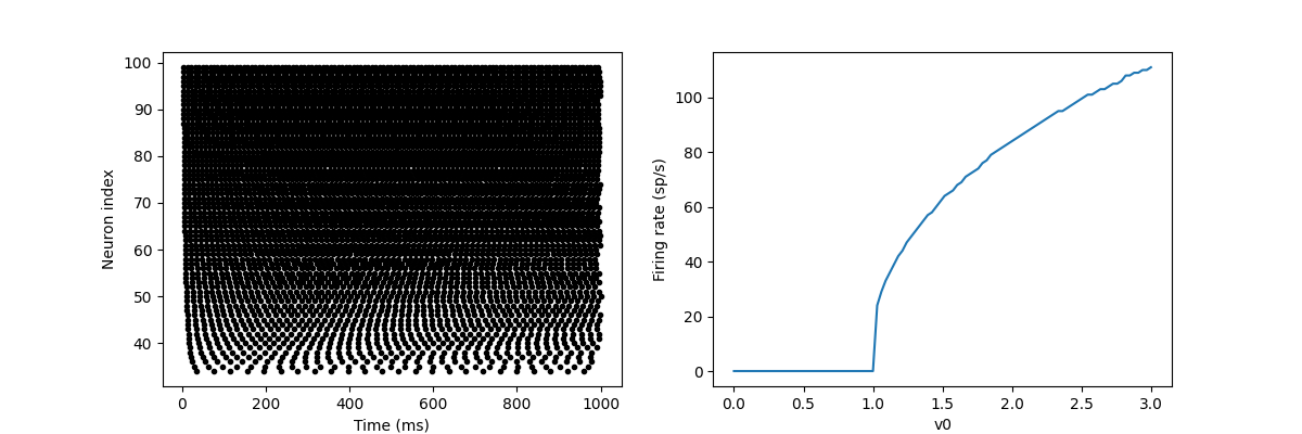
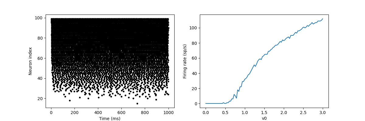
In this example, we drive the neuron to this value in a V0 exponential manner, but when v > 1, it triggers a spike and resets. The result is that the rate at which it emits the spike will be related to the value of v0. Because V0 < 1, it never emits spikes, and as V0 increases, it emits spikes at a higher rate. The right figure shows the ignition rate as a function of v0. This is the If curve of this neuron model.

Note that in the figure, we use the variable count in spike monitor: This is an array of the number of spikes excited by each neuron in the group. Divide it by the duration of operation to obtain the ignition rate.

from brian2 import *
start_scope()
N = 100
tau = 10*ms
v0_max = 3.
duration = 1000*ms
sigma = 0.2
eqs = '''
dv/dt = (v0-v)/tau+sigma*xi*tau**-0.5 : 1 (unless refractory)
v0 : 1
'''
G = NeuronGroup(N, eqs, threshold='v>1', reset='v=0', refractory=5*ms, method='euler')
M = SpikeMonitor(G)
G.v0 = 'i*v0_max/(N-1)'
run(duration)
figure(figsize=(12,4))
subplot(121)
plot(M.t/ms, M.i, '.k')
xlabel('Time (ms)')
ylabel('Neuron index')
subplot(122)
plot(G.v0, M.count/duration)
xlabel('v0')
ylabel('Firing rate (sp/s)')
show()

Of when making models of neurons, we include a random element to model the effect of various forms of neural noise. In Brian, we can do this by using the symbol Xi in differential equations. Strictly speaking, this symbol is a "stochastic differential" but you can sort of thinking of it as just a Gaussian random variable with mean 0 and standard deviation 1. We do have to take into account the way stochastic differentials scale with time, which is why we multiply it by tau**-0.5 in the equations below (see a textbook on stochastic differential equations for more details). Note that we also changed the method keyword argument to use 'euler' (which stands for the Euler-Maruyama method) ; the 'exact' method that we used earlier is not applicable to stochastic differential equations

I didn't understand this program, so I attached the original text. After reading some literature, I found that compared with the previous code, some noise was added in the neural network, making the ignition rate rise in an S-shaped way. The following is the operation result.