Data
Attribute information:
1) ID number
2) Diagnosis (M = malignant, B = benign)
Calculate 10 real value characteristics of each nucleus:
a) Radius (average distance from center to perimeter)
b) Texture (standard deviation of gray value)
c) Perimeter
d) Area
e) Smoothness (local variation of radius length)
f) Compactness (perimeter ^ 2 / area - 1.0)
g) Concavity (severity of the concave part of the profile)
h) Concave points (number of concave parts of the profile)
i) Symmetry
j) Fractal dimension ("shoreline approximation" - 1)
The mean, standard deviation and maximum of these features are calculated for each image, and 30 features are generated.
| diagnosis | M malignant B benign |
| radius_mean | Radius average |
| texture_mean | Texture average |
| perimeter_mean | Perimeter average |
| area_mean | Area average |
| smoothness_mean | Average smoothness |
| compactness_mean | Average tightness |
| concavity_mean | Average concavity |
| concave points_mean | Average value of concave joint |
| symmetry_mean | Symmetry average |
| fractal_dimension_mean | Average fractal dimension |
| radius_se | Standard deviation of radius |
| texture_se | Texture standard deviation |
| perimeter_se | Standard deviation of perimeter |
| area_se | Area standard deviation |
| smoothness_se | Standard deviation of smoothness |
| compactness_se | Standard deviation of tightness |
| concavity_se | Concavity standard deviation |
| concave points_se | Standard deviation of concave joint |
| symmetry_se | Symmetry standard deviation |
| fractal_dimension_se | Standard deviation of fractal dimension |
| radius_worst | Maximum radius |
| texture_worst | Texture Max |
| perimeter_worst | Perimeter Max |
| area_worst | Maximum area |
| smoothness_worst | Maximum smoothness |
| compactness_worst | Maximum tightness |
| concavity_worst | Concavity Max |
| concave points_worst | Maximum value of concave joint |
| symmetry_worst | Symmetry maximum |
| fractal_dimension_worst | Maximum fractal dimension |
1. Run pip install pyspark command to install the latest version of pyspark
!pip install pyspark
2. Import
The required packages are mainly pyspark machine learning packages such as pyspark.ml
import os
import pandas as pd
import numpy as np

from pyspark import SparkConf, SparkContext
from pyspark.sql import SparkSession, SQLContext

from pyspark.sql.types import *
import pyspark.sql.functions as F
from pyspark.sql.functions import udf, col

from pyspark.ml.regression import LinearRegression
from pyspark.mllib.evaluation import RegressionMetrics

from pyspark.ml.tuning import ParamGridBuilder, CrossValidator, CrossValidatorModel
from pyspark.ml.feature import VectorAssembler, StandardScaler
from pyspark.ml.evaluation import RegressionEvaluator
three Create a SparkSession object to use Spark
from pyspark.sql import SparkSession
spark = SparkSession.builder.master("local[2]").appName("breast-cancer-prediction").getOrCreate()

spark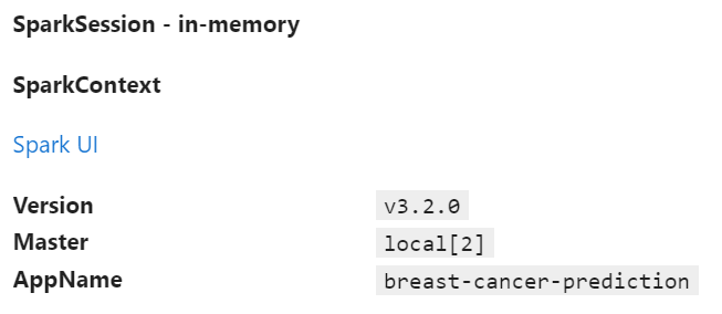
4. Read data set
df = spark.read.csv('../input/breast-cancer-wisconsin-data/data.csv',inferSchema=True,header=True)

df.show(3)
5. Analyze the label distribution of the data set
#View the shape structure of the dataset to determine the size of the dataset
print((df.count(),len(df.columns)))
#View the data type of the dataset
df.printSchema()
#The describe function views the statistical indicators of the dataset
df.describe().show(5,False)
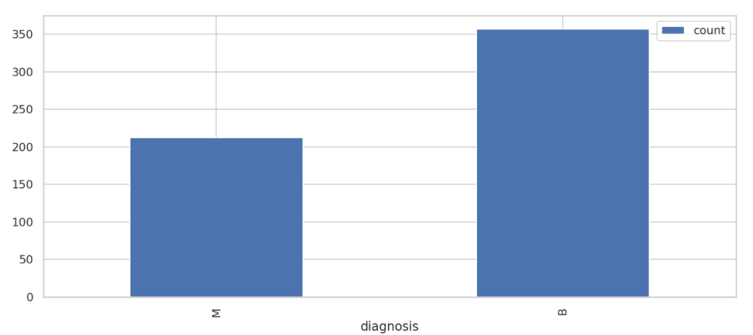
# Group by diagnostic results and view the distribution of results
result_df = df.groupBy("diagnosis").count().sort("diagnosis", ascending=False)
result_df.show()
result_df.toPandas().plot.bar(x='diagnosis',figsize=(14, 6))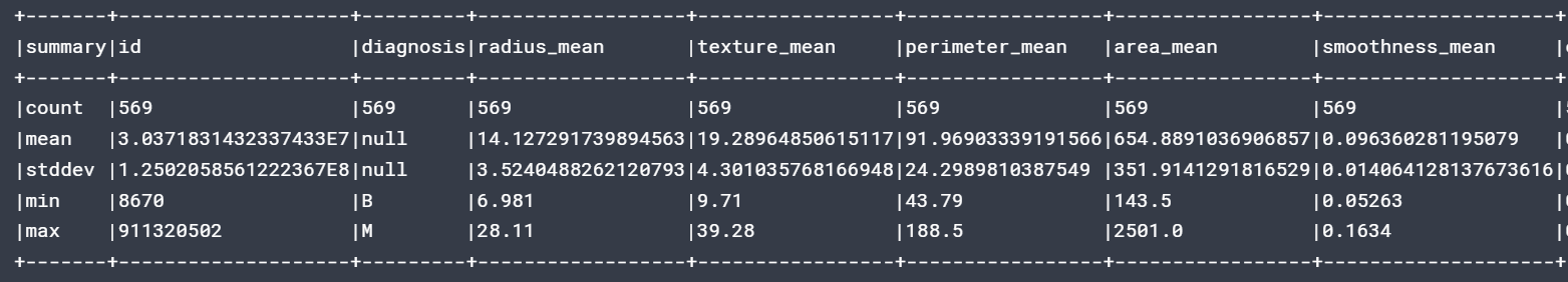
6. Data cleaning
Analyze the characteristic distribution of the data, and clean the missing values, error values and abnormal values in the data
#View the number of null values in each column
df_agg = df.agg(*[F.count(F.when(F.isnull(c), c)).alias(c) for c in df.columns])
df_agg.show()

#Delete c_32 columns
df=df.drop('_c32')

#Check the data type of the input column again. Only diagnosis is of string type, and all other columns are of numeric type
df.printSchema()

#Directly delete rows with missing values
#Process duplicate values
df = df.dropna()
df = df.dropDuplicates()
print((df.count(),len(df.columns)))
7. Characteristic Engineering
from pyspark.ml.linalg import Vector
from pyspark.ml.feature import VectorAssembler

#View column names
df.columns

#Represent features as vectors
vec_assembler = VectorAssembler(inputCols=['radius_mean','texture_mean','perimeter_mean', 'area_mean','smoothness_mean', 'compactness_mean','concavity_mean','concave points_mean','symmetry_mean','fractal_dimension_mean','radius_se','texture_se','perimeter_se','area_se', 'smoothness_se', 'compactness_se', 'concavity_se','concave points_se','symmetry_se', 'fractal_dimension_se', 'radius_worst', 'texture_worst','perimeter_worst', 'area_worst', 'smoothness_worst', 'compactness_worst', 'concavity_worst', 'concave points_worst', 'symmetry_worst','fractal_dimension_worst'],outputCol='features')
features_df = vec_assembler.transform(df)
features_df.printSchema()

features_df.select('features').show(3,truncate=False)

#Use StandardScaler to initialize features and output them to features_ In the scaled column
from pyspark.ml.feature import StandardScaler
standardScaler = StandardScaler(inputCol="features", outputCol="features_scaled")
scaled_df = standardScaler.fit(features_df).transform(features_df)
scaled_df.select("features", "features_scaled").show(1, truncate=False)

#Converts a character type diagnosis to a numeric type diagnosis_ The index value is 0,1
from pyspark.ml.feature import StringIndexer
diagnosis_index = StringIndexer(inputCol="diagnosis",outputCol="diagnosis_index").fit(scaled_df)

#Check the conversion results. The M malignant value is 1 and the B benign value is 0
scaled_df = diagnosis_index.transform(scaled_df)
model = scaled_df.select('diagnosis','diagnosis_index')
model.show(20)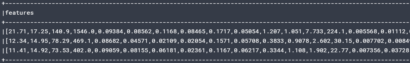
8. Divide data sets
train_df,test_df = scaled_df.randomSplit([0.8,0.2],seed=rnd_seed)

print((train_df.count(),len(train_df.columns)))
print((test_df.count(),len(test_df.columns)))
9. Logistic regression
Construct and train logistic regression model
from pyspark.ml.classification import LogisticRegression
from pyspark.ml import Pipeline
log_reg = LogisticRegression().setLabelCol("diagnosis_index").fit(train_df)

train_results = log_reg.evaluate(train_df).predictions
#The probability at index 0 is diagnosis_index = 0. The probability at the first index is diagnosis_index = 1 predicted
train_results.filter(train_results['diagnosis_index']==1).filter(train_results['prediction']==1).select(['diagnosis_index','prediction','probability']).show(20,False)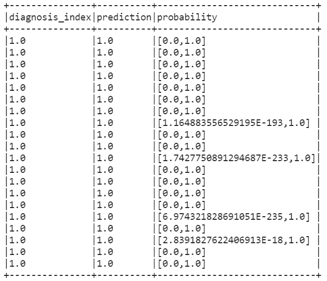
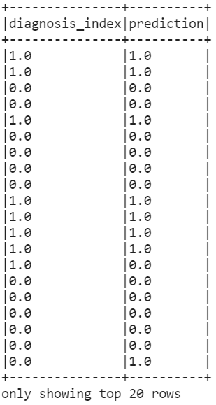
The logistic regression model was evaluated on the test data
results = log_reg.evaluate(test_df).predictions
results.printSchema()

results.select(['diagnosis_index','prediction']).show(20,False)
Classification model evaluation
1. Confusion matrix (with codes)
Confusion matrix is used to represent the error and measure the classification effect of the model. The matrix is a square matrix. The value of the matrix is used to represent the prediction results of the classifier, including correct positive prediction TP, positive negative prediction TN, wrong positive prediction FP and wrong negative prediction FN
2. Evaluation index (with codes)
- accuracy
- precision
- recall rate
- F1 (harmonic average)
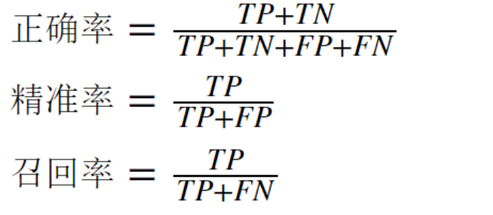
true_postives = results[(results.diagnosis_index == 1) & (results.prediction == 1)].count()
true_negatives = results[(results.diagnosis_index == 0) & (results.prediction == 0)].count()
false_positives = results[(results.diagnosis_index == 0) & (results.prediction == 1)].count()
false_negatives = results[(results.diagnosis_index == 1) & (results.prediction == 0)].count()

#Accuracy
accuracy=float((true_postives+true_negatives) /(results.count()))
print("accuracy:",accuracy)

#recall
recall = float(true_postives)/(true_postives + false_negatives)
print("recall:",recall)

#accuracy
precision = float(true_postives) / (true_postives + false_positives)
print("precision:",precision) 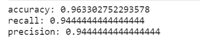
10. Random forest
#Constructing and training random forests
from pyspark.ml.classification import RandomForestClassifier
rf_classifier = RandomForestClassifier(labelCol='diagnosis_index',numTrees=50).fit(train_df)

#Evaluation based on test data
rf_predictions = rf_classifier.transform(test_df)
model = rf_predictions.select('diagnosis_index','prediction','probability')
model.show(10) 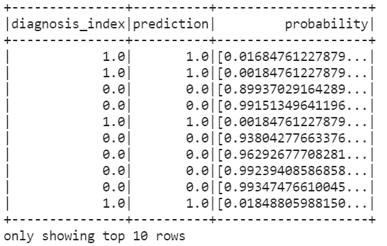
assessment
#assessment
from pyspark.ml.evaluation import MulticlassClassificationEvaluator
from pyspark.ml.evaluation import BinaryClassificationEvaluator

#Calculation accuracy
rf_accuracy = MulticlassClassificationEvaluator(predictionCol="prediction",labelCol='diagnosis_index',metricName='accuracy').evaluate(rf_predictions)
print('The accuracy of RF on test data is {0:.0%}'.format(rf_accuracy))

#Calculation accuracy
rf_precision = MulticlassClassificationEvaluator(labelCol='diagnosis_index',metricName='weightedPrecision').evaluate(rf_predictions)
print('The precision rate of RF on test data is {0:.0%}'.format(rf_precision)) 
AUC: AUC (Area Under the Curve) refers to the area under the ROC curve. The AUC value is used as the evaluation standard because the ROC curve can not clearly explain which classifier is better, and AUC as a value can intuitively evaluate the quality of the classifier. The larger the value, the better.
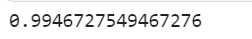
#Area under AUC ROC curve
from pyspark.ml.evaluation import BinaryClassificationEvaluator
rf_auc = BinaryClassificationEvaluator(labelCol='diagnosis_index').evaluate(rf_predictions)
print(rf_auc)