BFs

In fact, breadth-first search is hierarchical traversal, and the program is implemented by queue.

Algorithmic thought

Beginning with the root, the solution space tree of the problem is often searched by BF or in the way of minimum cost (i.e. maximum benefit) priority. Firstly, the root node is added to the live node table, and then the root node is extracted from the live node table to make it the current extended node. All the children's nodes are generated at one time to judge whether the children's nodes are abandoned or retained, which lead to infeasible solutions or non-optimal solutions, and the rest are retained in the live node table. Then a loopknot is taken from the loopknot table as the current extension node, and the extension process is repeated until the required solution is found or the loopknot table is space-time. Each live node has at most one chance to become an extended node.

Algorithm steps

The steps of solving the problem are as follows:

1. Define the solution space of the problem.
2. Determine the organizational structure of the solution space of the problem.
3. Search solution space. Before searching, criteria (constraint function or bound function) should be defined. If priority queue branch and bound method is selected, priority must be determined.

Similarities and Differences between Backtracking Method and Branch-and-Bound Method

1. Similarities:

• The solution space of the problem needs to be defined first, and the organization structure of the solution space is usually trees and graphs.
• Search the solution of the problem in the solution space tree.
• Before searching, it is necessary to determine the judgment condition, which is used to judge whether the node generated by the extension is a feasible node.
• In the process of searching, it is necessary to judge whether the node generated by the extension satisfies the judgment condition. If it satisfies, the extended node should be retained, otherwise it will be discarded.

2. different points

• The search objectives are different: the goal of backtracking is to find all the solutions satisfying the constraints in the solution space tree, while the goal of branch and bound method is to find a solution satisfying the constraints, or to find the optimal solution in a sense in the solution satisfying the constraints.
• Searching methods are different: backtracking searches spatial trees with depth-first search method, and branch-and-bound searches spatial trees with breadth-first search method or minimum consumption-first search method.
• Extension method is different: retrospective search, the extension node generates only one child node at a time, and branch and bound rule generates all child nodes at a time.

0-1 knapsack problem

problem analysis

There is, no more repetition.

w[]	1	2	3	4
2		5	4	2

v[]	1	2	3	4
6		3	5	4

The weight of the shopping cart W=10.
The structure of a commodity is defined as:

struct Goods
{
    int weight;
    int value;
} goods[N];

weight	2	5	4	2
value	6	3	5	4

Algorithm design

1. Define the solution space of the problem. The solution space of the problem is {x1,x2,...,xi,...,xn}, and the explicit constraint is xi=0 or 1.
2. Determine the organizational structure of solution space: subset tree.

3. Search solution space:

   • The constraints are: wixi < W (i=1~n)
   • Limit conditions: CP + rp > bestp (cp is the total value of the items currently loaded into the shopping cart, rp is the total value of the items from t+1 to n, and bestp is the maximum value)
4. Search process: Starting from the root node, search in BFS mode. The root node first becomes a live node, and it is also the current extension node. All child nodes are generated at one time. Since the value on the left branch is "1" in the subset tree, extending along the left branch of the extended node represents loading items; the value of the right branch is "0", representing not loading items. At this time, we can judge whether the constraints and boundaries are satisfied, and if they are satisfied, we will join them in the queue; otherwise, we will abandon them. Then an element is extracted from the queue as the current extension node, and the search process queue ends in space-time.

Step interpretation

1. Initialization. sumw=2+5+4+2=13, sumv=6+3+5+4=18, because sumw > W, so can not be loaded, so need to follow-up operation. Initialize cp=0,rp=sumv, current residual weight rw=W; current processing item serial number is 1; current optimal value bestp=0. Solution vector is x[]=(0,0,0,0), create a root node Node(cp,rp,rw,id), marked as A, add in FIFO queue q. CP is the value of the items loaded into the shopping cart, RP is the total value of the remaining items, RW is the residual capacity, ID is the item number, x [] is the current solution vector.

// Define nodes. Each node records the current solution.
struct Node

{
    int cp, rp; //Total value of cp knapsack items and total value of rp surplus items
    int rw; //Residual capacity
    int id; //Item number
    bool x[N];//Solution vector
    Node() {}
    Node(int _cp, int _rp, int _rw, int _id){
        cp = _cp;
        rp = _rp;
        rw = _rw;
        id = _id;
        memset(x, 0, sizeof(x));//Solution vector initialization is 0
    }
};

1. Extend node A. The head element A is in the queue, and the node's cp+rp (> bestp) satisfies the boundary condition and can be extended. RW = 10 > goods [1]. weight = 2, the remaining capacity greater than item 1, meet the constraints, can be put into the shopping cart, cp=0+6=6. rp=18-6=12, rw=10-2=8, t=2, x[1]=1, the solution vector is updated to x[]=(1,0,0,0), generating left child B, joining q queue, updating bestp=6. Then expand the right branch, CP = 0, rp=18-6=12, cp+rp > = bestp=6, satisfy the boundary conditions, do not put item 1, cp=0,rp=12,rw=10,t=2,x[1]=0, the solution vector is x[]=(0,0,0,0), create a new node C, join q queue. As shown in the table below, X is empty.

1. Extend B node. The head element B is out of the team, and the node cp+rp>=bestp satisfies the boundary condition and can be extended. RW = 8 > goods [2]. weight = 5, the remaining capacity is greater than the weight of item 2, meet the constraints, can be put into the shopping cart, cp=6+3=9. rp=12-3=9, rw=8-5=3, t=3, x[2]=1, the solution vector is updated to x[]=(1,1,0,0), generating left child D, joining q queue, updating bestp=9. Then expand the right branch, CP = 6, rp=12-3=9, CP + RP > = bestp=9, satisfy the boundary conditions, do not put item 2, cp=6,rp=9,rw=8,t=3,x[2]=0, the solution vector is x[]=(1,0,0,0), create a new node E, join the q queue. As shown in the table below.

1. Extend the C node. The head element C is in the queue, and the node cp+rp>= bestp satisfies the boundary condition and can be extended. RW = 10 > goods [2]. weight = 5, the remaining capacity is greater than the weight of item 2, meet the constraints, can be put into the shopping cart, cp=0+3=3. rp=12-3=9, rw=10-5=5, t=3, x[2]=1, the solution vector is updated to x[]=(0,1,0,0), generate left child F, join q queue. Then expand the right branch, CP = 0, rp=12-3=9, CP + RP > = bestp = 9, satisfy the boundary conditions, do not put item 2, cp=6,rp=9,rw=10,t=3,x[2]=0, the solution vector is x[]=(0,0,0,0), create a new node G, join the q queue. As shown in the table below.

1. Extend the D node. The head element D is out of the team, and the node cp+rp>=bestp satisfies the boundary condition and can be extended. But RW = 3 > goods [3]. weight = 4, so we do not meet the constraints and abandon the left branch. Expand the right branch, CP = 9, RP = 9-5 = 4, CP + RP > = bestp = 9, satisfy the boundary conditions, do not put item 3, cp=9,rp=4,rw=3,t=4,x[3]=0, the solution vector is x[]=(1,1,0,0), create a new node H, join the q queue. As shown in the table below.

1. Extend the E node. Similarly, we can get cp=11,rp=4,rw=4,t=4,x[3]=1, update the solution vector to x[]=(1,0,1,0), generate left child I, join q queue, update bestp=11. Extend the right branch, cp=6,rp=9-5=4,cp+rp=10
2. Extend the F node. Similarly, we get the left branch, cp=8,rp=4,rw=1,t=4,x[3]=1, and the solution vector is x[]=(0,1,1,0). We generate the left child J and join the q queue. Expand the right branch, CP + RP < 11, discard.
3. Extend the G node. The node cp+rp
4. Extend H node. The head H node is out of the queue. The node cp+rp>=bestp satisfies the boundary condition, rw=3>goods[4]. weight=2 satisfies the constraint condition, so that cp=9+4=13,rp=4-4=0,rw=3-2=1,t=5,x[4]=1, the solution vector is updated to x[]=(1,1,0,1), generates the child K, joins the q queue, and updates bestp=13. The right branch does not satisfy the boundary condition and is discarded.
5. Extend I node. The head I node is out of the queue. The node cp+rp>=bestp satisfies the boundary condition, rw=4>goods[4].weight=2 satisfies the constraint condition, so that cp=11+4=15,rp=4-4=0,rw=4-2=2,t=5,x[4]=1, the solution vector is updated to x[]=(1,0,1,1), generates the child L, joins the q queue, and updates bestp=15. The right branch does not satisfy the boundary condition and is discarded.
6. The head element J is out of the team, and the node cp+rp=12<15 does not satisfy the boundaries and does not expand any more.
7. Team leader element K out, extended K node: t=5, has been processed, cp
8. The head element K is out of the queue, extending K node: t=5, has been processed, cp=bestp, is the optimal solution, output the vector (1, 0, 1, 1).
9. The queue is empty and the algorithm ends.

code implementation

int bestp, W, n, sumw, sumv;
/*
bestp Used to record the optimal solution.
W Maximum capacity for shopping carts.
n Number of items.
sumw For the total weight of all items.
sumv For the total value of all items.
*/
//bfs searches the subset tree.
int bfs()
{
    int t, tcp, trp, trw;
    queue<Node> q; //Create a regular queue (FIFO)
    q.push(Node(0, sumv, W, 1)); //Press into an initial node
    while (!q.empty()) //If the queue is not empty
    {
        Node livenode, lchild, rchild;//Define three nodal variables
        livenode = q.front();//Remove the header element as the current extended node livenode
        q.pop(); //Team Leader Element Out
                 //CP + RP > bestp is no longer extended when the current loading value + the value of surplus items is less than the current optimal value.
        cout << "Current Node id value:" << livenode.id << "Current Node cp value:" << livenode.cp << endl;
        cout << "Solution Vector of Current Node:";
        for (int i = 1; i <= n; i++)
        {
            cout << livenode.x[i];
        }
        cout << endl;
        t = livenode.id;//Item Number of Current Processing
                        // You don't need to search down when you find the last item.
                        // If the current shopping cart has no surplus capacity, it will not expand.
        if (t>n || livenode.rw == 0)
        {
            if (livenode.cp >= bestp)//Updating the Optimal Solution and Value
            {
                for (int i = 1; i <= n; i++)
                {
                    bestx[i] = livenode.x[i];
                }
                bestp = livenode.cp;
            }
            continue;
        }
        if (livenode.cp + livenode.rp<bestp)//Determine whether the current node satisfies the boundary condition, if it does not meet the extension
            continue;
        //Expanding Left Child
        tcp = livenode.cp; //Value in the Current Shopping Cart
        trp = livenode.rp - goods[t].value; //Whether the current item is loaded or not, the surplus value will decrease.
        trw = livenode.rw; //Remaining capacity of shopping cart
        if (trw >= goods[t].weight) //Satisfies the restriction condition, may put in the shopping cart
        {
            lchild.rw = trw - goods[t].weight;
            lchild.cp = tcp + goods[t].value;
            lchild = Node(lchild.cp, trp, lchild.rw, t + 1);//Transfer parameters
            for (int i = 1; i<t; i++)
            {
                lchild.x[i] = livenode.x[i];//Reproduce the previous solution vector
            }
            lchild.x[t] = true;
            if (lchild.cp>bestp)//Update more than the optimal value
                bestp = lchild.cp;
            q.push(lchild);//Left Children Enter the Team
        }
        //Expanding Right Child
        if (tcp + trp >= bestp)//Do not put in shopping cart to meet the limit conditions
        {
            rchild = Node(tcp, trp, trw, t + 1);//Transfer parameters
            for (int i = 1; i<t; i++)
            {
                rchild.x[i] = livenode.x[i];//Replicate the previous solution vector
            }
            rchild.x[t] = false;
            q.push(rchild);//The right child joins the team
        }
    }
    return bestp;//Returns the optimal value.
}

algorithm analysis

The time complexity is O(2n+1) and the space complexity is O(n*2n+1).

Optimal Extension of Algorithms-Priority Queuing Branch-and-Bound Method

Priority queue optimization simply means that the upper bound of the current node is taken as the priority value and the ordinary queue is changed into the priority queue.

1. Algorithmic design. The constraints remain unchanged. Priority is defined as the upper bound of the value of the loaded item represented by the partial unlocking of the loose node. The higher the upper bound of the value, the higher the priority. The upper bound of the value of the live node is up = the maximum value rp', where the cp + surplus of the live node is filled with the remaining capacity of the shopping cart. The limit condition becomes up = cp + rp'> = bestp.

2. Problem Solving Steps (Brief Edition)

   • Initialization. Sumw and sumv are used to calculate the total weight and value of all items respectively. Sumw = 13, sumv = 18, sumw > W, so it can not be all loaded, need to search and solve.
   • The order is non-incremental according to the ratio of value to weight. The sorting results are shown in the table below.
   • No further details will be given.

weight	2	2	4	5
value	6	4	5	3

3. Code Implementation

//Define the structure of auxiliary items, including the serial number of items and the value of unit weight, for sorting by unit weight value (value/weight ratio).
struct Object
 {
        int id; //Item serial number
        double d;//Unit weight value
    }S[N];
    
//Define the priority of sorting according to the unit weight value of the item from big to small
bool cmp(Object a1,Object a2)
{
    return a1.d>a2.d;
}

//Define the priority of the queue. With up as the priority, the higher the up value, the higher the priority.
bool operator <(const Node &a, const Node &b)
{
    return a.up<b.up;
}

int bestp,W,n,sumw,sumv;
/*
  bestv Used to record the optimal solution.
  W For the maximum capacity of the backpack.
  n For the number of items.
  sumw For the total weight of all items.
  sumv For the total value of all items.
*/

double Bound(Node tnode)
{
    double maxvalue=tnode.cp;//Value of items loaded into shopping carts
    int t=tnode.id;//Ordinal number after sorting
    //cout<<"t="<<t<<endl;
    double left=tnode.rw;//Residual capacity
    while(t<=n&&w[t]<=left)
    {
        maxvalue+=v[t];
       // cout<<"malvalue="<<maxvalue<<endl;
        left-=w[t];
        t++;
    }
    if(t<=n)
        maxvalue+=double(v[t])/w[t]*left;
    //cout<<"malvalue="<<maxvalue<<endl;
    return maxvalue;
}
//priorbfs is a priority queue branch and bound search method.
int priorbfs()
{
     int t,tcp,trw;
     double tup; //The item number t currently processed, the item value tcp currently loaded into the shopping cart,
    //The upper bound tup of the value of the goods currently loaded into the shopping cart, the current remaining capacity trw
    priority_queue<Node> q; //Create a priority queue with priority as the up per bound of the value of the item loaded into the shopping cart
    q.push(Node(0, sumv, W, 1));//Initialization, root node joins priority queue
    while(!q.empty())
    {
        Node livenode, lchild, rchild;//Define three nodal variables
        livenode=q.top();//Remove the header element as the current extended node livenode
        q.pop(); //Team Leader Element Out
        cout<<"Current Node id value:"<<livenode.id<<"Current Node up value:"<<livenode.up<<endl;
        cout<<"Solution Vector of Current Node:";
        for(int i=1; i<=n; i++)
        {
            cout<<livenode.x[i];
        }
        cout<<endl;
        t=livenode.id;//Item Number of Current Processing
        // You don't need to search down when you find the last item.
        // If the current shopping cart has no surplus capacity, it will not expand.
        if(t>n||livenode.rw==0)
        {
            if(livenode.cp>=bestp)//Updating the Optimal Solution and Value
            {
              cout<<"Updating the Optimal Solution Vector:";
              for(int i=1; i<=n; i++)
              {
                bestx[i]=livenode.x[i];
                cout<<bestx[i];
              }
              cout<<endl;
              bestp=livenode.cp;
            }
            continue;
        }
        //Determine whether the current node satisfies the boundary condition, if it does not meet the extension
        if(livenode.up<bestp)
          continue;
        //Expanding Left Child
        tcp=livenode.cp; //Value in the Current Shopping Cart
        trw=livenode.rw; //Remaining capacity of shopping cart
        if(trw>=w[t]) //Satisfies the restriction condition, may put in the shopping cart
        {
            lchild.cp=tcp+v[t];
            lchild.rw=trw-w[t];
            lchild.id=t+1;
            tup=Bound(lchild); //Calculate the upper bound of the left child
            lchild=Node(lchild.cp,tup,lchild.rw,lchild.id);//Transfer parameters
            for(int i=1;i<=n;i++)
            {
              lchild.x[i]=livenode.x[i];//Replicate the previous solution vector
            }
            lchild.x[t]=true;
            if(lchild.cp>bestp)//Update more than the optimal value
               bestp=lchild.cp;
            q.push(lchild);//Left Children Enter the Team
        }
        //Expanding Right Child
         rchild.cp=tcp;
         rchild.rw=trw;
         rchild.id=t+1;
         tup=Bound(rchild); //Right child calculates upper bound
         if(tup>=bestp)//Do not put in shopping cart to meet the limit conditions
         {
            rchild=Node(tcp,tup,trw,t+1);//Transfer parameters
            for(int i=1;i<=n;i++)
            {
              rchild.x[i]=livenode.x[i];//Reproduce the previous solution vector
            }
            rchild.x[t]=false;
            q.push(rchild);//The right child joins the team
          }
    }
    return bestp;//Returns the optimal value.
}

traveling salesman problem

problem analysis

The weighted adjacency matrix g [][] is shown below. The null is expressed as infinite, i.e. there is no path.

	15	30	5
15		6	12
30	6		3
5	12	3

Algorithm design

The priority queue branch and bound method can be used to speed up the search.
Priority setting: All path lengths CL of the cities currently traveled. The smaller the cl, the higher the priority.
Starting from the root node, the search is carried out in a breadth-first manner. The root node first becomes a live node, and it is also the current extension node. Generate all the children's nodes at one time, judge whether the children's nodes meet the constraints and boundaries, if satisfied, add them to the queue, otherwise, abandon them. Then an element is extracted from the queue as the current extension node, and the search process queue is listed as space-time.

code implementation

struct Node//Define the node and record the solution information of the current node
{
    double cl; //Currently traveled path length
    int id; //Serial number of scenic spots
    int x[N];//Record the current path
    Node() {}
    Node(double _cl,int _id)
    {
        cl = _cl;
        id = _id;
    }
};

//Define the priority of the queue. With cl as the priority, the smaller the cl value, the more priority
bool operator <(const Node &a, const Node &b)
{
    return a.cl>b.cl;
}

//Traveling BFS search for priority queue branch and bound method
double Travelingbfs()
{
    int t; //The number t of the attractions currently being processed
    Node livenode,newnode;//Define the current extended node livenode to generate a new node
    priority_queue<Node> q; //Create a priority queue with priority to the path length CL that has been traveled. The smaller the CL value, the higher the priority.
    newnode=Node(0,2);//Create the root node
    for(int i=1;i<=n;i++)
    {
       newnode.x[i]=i;//Solution Vector of Initialized Root Node
    }
    q.push(newnode);//Root node joins priority queue
    cout<<"In priority order:"<<endl;//For debugging
    while(!q.empty())
    {
        livenode=q.top();//Remove the header element as the current extended node livenode
        q.pop(); //Team Leader Element Out
        //For debugging
        cout<<"Current Node id value:"<<livenode.id<<"Current Node cl value:"<<livenode.cl<<endl;
        cout<<"Solution Vector of Current Node:";
        for(int i=1; i<=n; i++)
        {
            cout<<livenode.x[i];
        }
        cout<<endl;
        t=livenode.id;//Number of attractions currently being processed
        // You don't need to search down when you find the last two spots
        if(t==n)  //Judge immediately whether to update the optimal solution.
            //For example, a path (1243) is currently found, and when it reaches Node 4, it is immediately judged whether g[4][3] and g[3][1] are edged connected.
            //If there are edges, the current path length Cl + G [4] [3] + G [3] [1] < bestl is judged, and the optimal value and solution are updated if satisfied.
        {
           //It shows that we have found a better way to record relevant information.
           if(g[livenode.x[n-1]][livenode.x[n]]!=INF&&g[livenode.x[n]][1]!=INF)
             if(livenode.cl+g[livenode.x[n-1]][livenode.x[n]]+g[livenode.x[n]][1]<bestl)
             {
                bestl=livenode.cl+g[livenode.x[n-1]][livenode.x[n]]+g[livenode.x[n]][1];
                cout<<endl;
                cout<<"The Current Optimal Solution Vector:";
                for(int i=1;i<=n;i++)
                {
                  bestx[i]=livenode.x[i];
                  cout<<bestx[i];
                }
                cout<<endl;
                cout<<endl;
              }
            continue;
        }
        //Determine whether the current node satisfies the boundary condition, if it does not meet the extension
       if(livenode.cl>=bestl)
          continue;
        //extend
        //Not reaching the leaf node
        for(int j=t; j<=n; j++)//Search for all branches of extended nodes
        {
            if(g[livenode.x[t-1]][livenode.x[j]]!=INF)//If x[t-1] attractions are connected side by side with x[j] attractions
            {
                double cl=livenode.cl+g[livenode.x[t-1]][livenode.x[j]];
                if(cl<bestl)//It's possible to get shorter routes.
                {
                    newnode=Node(cl,t+1);
                    for(int i=1;i<=n;i++)
                    {
                      newnode.x[i]=livenode.x[i];//Replicate the previous solution vector
                    }
                    swap(newnode.x[t], newnode.x[j]);//Exchange the values of two elements x[t], x[j]
                    q.push(newnode);//New Node Entry
                }
            }
        }
    }
    return bestl;//Returns the optimal value.
}

(1) Time complexity: O(n!). Spatial complexity: O(n*n!).

Extension of algorithm optimization

1. The algorithm starts by creating a queue that represents a live node priority. The lower cost bound zl=cl+rl value of each node is taken as priority. cl denotes the path length that has been traveled, rl denotes the lower bound of the remaining path length, rl is calculated by the sum of the minimum outgoing edges of each remaining node. Initially, the minimum outgoing edges of each vertex i in the graph are computed, and recorded with minout[i] array. minsum records the sum of the minimum outgoing edges of all nodes. If a vertex in the given digraph has no edge, the graph can not have a loop and the algorithm ends immediately.

   • Limit condition: zl
2. Priority: ZL refers to the lower bound of the path length that has been traveled + the remaining path length. The smaller the zl, the higher the priority.

Algorithmic optimization code implementation

1. Define Node Structures

//Define the node and record the solution information of the current node
struct Node
{
    double cl; //Currently traveled path length
    double rl; //Lower bound of residual path length
    double zl; //The lower bound of the current path length zl=rl+cl
    int id; //Serial number of scenic spots
    int x[N];//Record the current solution vector
    Node() {}
    Node(double _cl,double _rl,double _zl,int _id)
    {
        cl = _cl;
        rl = _rl;
        zl = _zl;
        id = _id;
    }
};

2. Defining queue priority

bool operator <(const Node &a, const Node &b)
{
    return a.zl>b.zl;
}

3. Computational lower bound

bool Bound()//Calculate the lower bound (that is, the sum of the minimum outbound weights for each scenic spot)
{
    for(int i=1;i<=n;i++)
    {
       double minl=INF;//Minimum Outside Points of Initial Scenic Spots
       for(int j=1;j<=n;j++)//Find the smallest way out of every scenic spot
         if(g[i][j]!=INF&&g[i][j]<minl)
            minl=g[i][j];
       if(minl==INF)
          return false;//Represents no loop
       minout[i]=minl;//Record the minimum outbound of each scenic spot
       cout<<"The first"<<i<<"Minimum number of attractions:"<<minout[i]<<" "<<endl;
       minsum+=minl;//Record the minimum outbound sum of all scenic spots
    }
    cout<<"The sum of the minimum outbound of each scenic spot:""minsum= "<<minsum<<endl;
    return true;
}

4. Traveling bfsopt as an optimized priority queue branch-and-bound method

double Travelingbfsopt()
{
    if(!Bound())
        return -1;//Represents no loop
    Node livenode,newnode;//Define the current extended node livenode to generate a new node
    priority_queue<Node> q; //Create a priority queue with the lower bound ZL = RL + Cl of the current path length as the priority. The smaller the ZL value, the higher the priority.
    newnode=Node(0,minsum,minsum,2);//Create the root node
    for(int i=1;i<=n;i++)
    {
       newnode.x[i]=i;//Solution Vector of Initialized Root Node
    }
    q.push(newnode);//Root node joins priority queue
    while(!q.empty())
    {
        livenode=q.top();//Remove the header element as the current extended node livenode
        q.pop(); //Team Leader Element Out
        cout<<"Current Node id value:"<<livenode.id<<"Current Node zl value:"<<livenode.zl<<endl;
        cout<<"Solution Vector of Current Node:";
        for(int i=1; i<=n; i++)
        {
            cout<<livenode.x[i];
        }
        cout<<endl;
        int t=livenode.id;//Number of attractions currently being processed
        // You don't need to search down when you find the last two spots
        if(t==n)  //Judge immediately whether to update the optimal solution.
            //For example, a path (1243) is currently found, and when it reaches Node 4, it is immediately judged whether g[4][3] and g[3][1] are edged connected.
            //If there are edges, the current path length Cl + G [4] [3] + G [3] [1] < bestl is judged, and the optimal value and solution are updated if satisfied.
        {
           //It shows that we have found a better way to record relevant information.
           if(g[livenode.x[n-1]][livenode.x[n]]!=INF&&g[livenode.x[n]][1]!=INF)
             if(livenode.cl+g[livenode.x[n-1]][livenode.x[n]]+g[livenode.x[n]][1]<bestl)
             {
                bestl=livenode.cl+g[livenode.x[n-1]][livenode.x[n]]+g[livenode.x[n]][1];
                cout<<endl;
                cout<<"The Current Optimal Solution Vector:";
                for(int i=1;i<=n;i++)
                {
                  bestx[i]=livenode.x[i];
                  cout<<bestx[i];
                }
                cout<<endl;
                cout<<endl;
              }
            continue;
        }
        //Determine whether the current node satisfies the boundary condition, if it does not meet the extension
       if(livenode.cl>=bestl)
          continue;
        //extend
        //Not reaching the leaf node
        for(int j=t; j<=n; j++)//Search for all branches of extended nodes
        {
            if(g[livenode.x[t-1]][livenode.x[j]]!=INF)//If x[t-1] attractions are connected side by side with x[j] attractions
            {
                double cl=livenode.cl+g[livenode.x[t-1]][livenode.x[j]];
                double rl=livenode.rl-minout[livenode.x[j]];
                double zl=cl+rl;
                if(zl<bestl)//It's possible to get shorter routes.
                {
                    newnode=Node(cl,rl,zl,t+1);
                    for(int i=1;i<=n;i++)
                    {
                      newnode.x[i]=livenode.x[i];//Replicate the previous solution vector
                    }
                    swap(newnode.x[t], newnode.x[j]);//Exchange the values of two elements
                    q.push(newnode);//New Node Entry
                }
            }
        }
    }
    return bestl;//Returns the optimal value.
}

Algorithmic complexity analysis

The worst time complexity is O (n n!) and the worst space complexity is O(n2*(n+1)!).

Optimal Engineering Routing Problem

Problem description

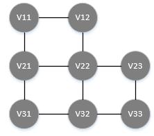
In 3 *3 square array, gray means blockade and can not pass. Each grid is abstracted as a node. The grid and the passing grid in four directions (up and down or left) are connected by a line, and the passing grid is not connected. In this way, the solution space of the problem can be defined as a graph, as shown in the following figure.

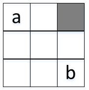
This problem is a special shortest path problem. The special point is that the number of squares traveled by the routing represents the length of the routing. When routing, the length of each square is added up to 1. We can see that there are many routing schemes from a to b. The shortest routing length is the shortest path length from a to b which is 4.
Since it can only be routed in four directions, that is to say, from the perspective of tree search, we can regard it as an m-fork tree, then the solution space of the problem becomes an m-fork tree.

Algorithm design

(1) Define the solution space of the problem. The optimal engineering routing problem can be solved i n the form of N tuple {x1, x2,..., x i,..., x n}, component X I represents the first square through which the optimal routing scheme passes, and the lattice can also be expressed i n the form of (x,y) row X and column y. Because the grid can not be repeated wiring, so in determining xi, the previous passing grid {x1,x2,...,xi-1} can not go any further. The value range of Xi is S-{x1,x2,...,xi-1}.
Note: Unlike the previous problem, n is unknown because the optimal wiring length is unknown.

(2) The organizational structure of solution space: a m-fork tree, m=4, the depth of the tree is unknown.

(3) Search solution space. The search starts at the starting node a and ends at the target node b.

• Constraints: no barrier or boundary wiring.
• Limit condition: The first condition to be encountered must be the shortest distance, so the infinite boundary condition.
• Search process: Starting from a, it is regarded as the first extension node and expands along the adjacent nodes in the right, lower, left and upper directions of A. To determine whether the constraints are valid, if they are valid, they are put into the live node and marked as 1. Then, the first node of the queue is taken as the next extension node, and the adjacent nodes are expanded along the four directions of the current expansion node: right, lower, left and upper. The grid satisfying the constraints is marked as 2. By analogy, the search is continued until the target grid or the live node is empty, and the data in the target grid is the optimal routing length.

The process of constructing the optimal solution starts from the target node and follows the four directions of right, bottom, left and top. It is judged that if the data in a direction grid is 1 less than that in an extended node grid, it will enter the direction grid and make it the current extended node. By analogy, the search process lasts until the end of the starting node.

Algorithm implementation

//Define structure position
typedef struct
{
    int x;
    int y;
} Position;//position
int grid[100][100];//Map
bool findpath(Position s, Position e, Position *&path, int &PathLen)
{
    if ((s.x == e.x) && (s.y == e.y))//The starting position is the ending position.
    {
        PathLen = 0;
        return true;
    }
    Position DIR[4], here, next;
    //Define Direction Array DIR[4], Current Location here, next Location
    DIR[0].x = 0;
    DIR[0].y = 1;
    DIR[1].x = 1;
    DIR[1].y = 0;
    DIR[2].x = 0;
    DIR[2].y = -1;
    DIR[3].x = -1;
    DIR[3].y = 0;
    here = s;
    grid[s.x][s.y] = 0;//The initial mark is 0, the unpacked line is - 1, and the wall is - 2.
    queue<Position> Q;//Queues used
    //Search in four directions
    for (;;)
    {
        for (int i = 0; i < 4; i++)//Go in four directions, right down, left up
        {
            next.x = here.x + DIR[i].x;
            next.y = here.y + DIR[i].y;
            if (grid[next.x][next.y] == -1)//No wiring
            {
                grid[next.x][next.y] = grid[here.x][here.y] + 1;
                Q.push(next);
            }
            if ((next.x == e.x) && (next.y == e.y))
                break;//Find the goal we need
        }
        if ((next.x == e.x) && (next.y == e.y))
            break;//Find the goal we need
        if (Q.empty())
            return false;
        else
        {
            here = Q.front();
            Q.pop();//Pop out the elements of Q team head
        }
    }
    //Reverse Minimum Routing Scheme
    PathLen = grid[e.x][e.y];//Minimum length
    path = new Position[PathLen];
    here = e;
    for (int j = PathLen - 1; j >= 0; j--)
    {
        path[j] = here;
        //Look in four directions, lower right and upper left
        for (int i = 0; i < 4; i++)
        {
            next.x = here.x + DIR[i].x;
            next.y = here.y + DIR[i].y;
            if (grid[next.x][next.y] == j)
                break;
        }
        here = next;
    }
    return true;
}
//Initialize the map with a mark greater than 0 indicating that it has been wired, - 1 not wired, - 2 walls
void init(int m, int n)
{
    for (int i = 1; i <= m; i++)
        for (int j = 1; j <= n; j++)
            grid[i][j] = -1;
    //The above is to initialize all the lattices to -1 first.
    //Then, for the convenience of this problem, the 0th row and the 0th column are set as walls.
    for (int i = 0; i <= n + 1; i++)
        grid[0][i] = grid[m + 1][i] = -2;
    for (int i = 0; i <= m + 1; i++)
        grid[i][0] = grid[i][n + 1] = -2;
}

Complexity analysis

Time complexity O (nano), space complexity O(n) and O(L) are needed to construct the shortest routing.