1, Experimental purpose
This experiment aims to let students have a preliminary understanding of pattern recognition and have a deep understanding of Bayesian classification algorithm according to their own design
2, Experimental principle
1. Bayesian classification algorithm
Bayesian classification algorithm is a classification method of statistics. It is a kind of classification algorithm using probability and statistical knowledge. On many occasions, Na ï ve Bayes (NB) classification algorithm can be compared with decision tree and neural network classification algorithm. This algorithm can be applied to large databases, and has the advantages of simple method, high classification accuracy and fast speed.
2. Several algorithms
The purpose of this experiment is to let students have a preliminary understanding of pattern recognition and be able to
The design has a deep understanding of Bayesian classification algorithm.
A. Naive Bayesian algorithm
Let each data sample use an n-dimensional eigenvector to describe the values of N attributes, that is, X={x1, x2,..., xn}. Suppose there are m classes, represented by C1, C2,..., Cm respectively. Given an unknown data sample x (i.e. no class label), if the naive Bayesian classification assigns the unknown sample x to class Ci, it must be
P(Ci|X)>P(Cj|X) 1≤j≤m,j≠i
According to Bayes theorem
Since P(X) is constant for all classes, the maximum a posteriori probability P(Ci|X) can be transformed into the maximum a posteriori probability P(X|Ci)P(Ci). If the training data set has many attributes and tuples, the overhead of calculating P(X|Ci) may be very large. Therefore, it is usually assumed that the values of each attribute are independent of each other
A priori probabilities P(x1|Ci), P(x2|Ci),..., P(xn|Ci) can be obtained from the training data set.
According to this method, for sample X of an unknown category, the probability P(X|Ci)P(Ci) that x belongs to each category Ci can be calculated respectively, and then the category with the highest probability can be selected as its category.
The premise of naive Bayesian algorithm is that the attributes are independent of each other. When the data set meets this independence assumption, the classification accuracy is high, otherwise it may be low. In addition, the algorithm has no classification rule output.
B. TAN algorithm (tree enhanced naive Bayesian algorithm)
TAN algorithm reduces the assumption of independence between any attribute in NB by discovering the dependency between attribute pairs. It is realized by adding the Association (edge) between attribute pairs on the basis of Nb network structure.
The implementation method is: using nodes to represent attributes, using directed edges to represent the dependencies between attributes, taking category attributes as the root node, and all other attributes as its child nodes. Generally, dotted lines are used to represent the edges required by NB, and solid lines are used to represent the new edges. The edge between attribute Ai and Aj means that the influence of attribute Ai on category variable C also depends on the value of attribute Aj.
These added edges need to meet the following conditions: the category variable has no parent node, and each attribute has one category variable parent node and at most another attribute as its parent node.
After finding this group of associated edges, the joint probability distribution of a group of random variables can be calculated as follows:
among Π Ai represents the parent node of Ai. Because the association between (n-1) two attributes of N attributes is considered in TAN algorithm, the assumption of independence between attributes is reduced to a certain extent, but there may be more other associations between attributes, so its scope of application is still limited.
3, Experimental content
The classification is determined using Bayesian posterior probability:
4, Experimental code
M=50;% M Is the maximum number of classes
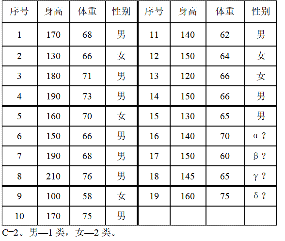
% 15 samples of known categories (height, weight, category). one-Male, 2-female
n=15;
pattern=[170,68,1;
130,66,2;
180,71,1;
190,73,1;
160,70,2;
150,66,1;
190,68,1;
210,76,1;
100,58,2;
170,75,1;
140,62,1;
150,64,2;
120,66,2;
150,66,1;
130,65,1];
% 4 samples of unknown category
X= [140,70,0;
150,60,0;
190,68,0;
160,75,0];
K=4; % Number of samples of unknown category
pattern % display pattern
X % Show samples of unknown categories
C=2; % Total categories C=2
num=zeros(1,C);
%array num(i)Storage section i Number of samples for class(i=1...C
for i=1:n % Count the number of samples of each type
num(pattern(i,3))=num(pattern(i,3))+1;
end
for i=1:C % Output samples of each type
fprintf('%d Number of class samples= %d \n',i,num(i))
end
% Calculate the a priori probability of each class
for i=1:C
P(i)=num(i)/n;
% Output a priori probability of each class
fprintf('%d A priori probability of class=%.2f \n',i,P(i))
end
% float PW1[M],PW2[M]; Store a posteriori probability array
% float height,weight; height-weight
% Classify and judge samples of unknown categories
for k=1:K % Sample data for unknown category: height-Weight to deal with
fprintf('The first%d Samples:%d,%d\n',k,X(k,1),X(k,2))
height=X(k,1);
weight=X(k,2);
num1=0;
for i=1:n
if (pattern(i,1)==height&pattern(i,3)==1)
num1=num1+1;
end
end
if (num1==0) % To prevent 0 probability, both numerator and denominator are processed: numerator plus 1, denominator plus category number or number of different values
PW1(1)=1/(num(1)+2);
else
PW1(1)=(num1+1)/(num(1)+2);
end
num1=0;
for i=1:n
if (pattern(i,2)==weight&pattern(i,3)==1)
num1=num1+1;
end
end
if (num1==0) % To prevent 0 probability, both numerator and denominator are processed: numerator plus 1, denominator plus category number or number of different values
PW1(2)=1/(num(1)+2);
else
PW1(2)=(num1+1)/(num(1)+2);
end
num2=0;
for i=1:n
if (pattern(i,1)==height&pattern(i,3)==2)
num2=num2+1;
end
end
if (num2==0)
PW2(1)=1/(num(2)+2);
else
PW2(1)=(num2+1)/(num(2)+2);
end
num2=0;
for i=1:n
if (pattern(i,2)==weight&pattern(i,3)==2)
num2=num2+1;
end
end
if (num2==0)
PW2(2)=1/(num(2)+2);
else
PW2(2)=(num2+1)/(num(2)+2);
end
PWT1=PW1(1)*PW1(2)*P(1); % Calculate the likelihood probability belonging to the first category*A priori probability
PWT2=PW2(1)*PW2(2)*P(2); % Calculate the likelihood probability belonging to the second category*A priori probability
fprintf(' Likelihood probability belonging to the first category*A priori probability (a posteriori probability)*P(X))= %.2f \n',PWT1)
fprintf(' Likelihood probability belonging to the second category*A priori probability (a posteriori probability)*P(X))= %.2f \n',PWT2)
if (PWT1>PWT2)
fprintf(' %d -th pattern belongs to 1\n',k)
elseif (PWT1<PWT2)
fprintf(' %d -th pattern belongs to 2\n',k)
else
fprintf(' %d -th pattern belongs to 1 or 2 is equal\n',k)
end
end