sort

1. Concept of sorting

Sorting: the so-called sorting is the operation of arranging a string of records incrementally or decrementally according to the size of one or some keywords.

Stability: if there are multiple records with the same keyword in the record sequence to be sorted, the relative order of these records remains unchanged after sorting, that is, in the original sequence, r[i]=r[j], and r[i] is before r[j], while in the sorted sequence, r[i] is still before r[j], then this sorting algorithm is said to be stable; Otherwise, it is called unstable.

Internal sorting: sorting in which all data elements are placed in memory.

External sorting: there are too many data elements to be placed in memory at the same time. According to the requirements of the sorting process, the sorting of data cannot be moved between internal and external memory.

2. Common sorting algorithms

• Insert sort: directly insert sort and insert sort
• Select sort: select sort and heap sort
• Swap sort: bubble sort, quick sort
• Merge sort: merge sort
• Non comparison sort: count sort

When writing sorting, first think about the writing method of one-time sorting, and then write the logic of multiple times.

2.1 insert sort

2.1.1 direct insertion sort

Basic idea: insert the records to be sorted into an ordered sequence one by one according to the size of their key values, until all records are inserted, and a new ordered sequence is obtained. [it is conceivable that when playing poker, insert the new card into the already arranged hand]

Insert sorting procedure directly:

When inserting the I (I > = 1) th element, the preceding array[0],array[1],..., array[i-1] have been arranged in order. At this time, compare the sorting code of array[i] with the sorting code of array[i-1],array[i-2],... To find the insertion position, that is, insert array[i], and move the element order at the original position backward

• Single pass sorting: insert x into the ordered interval of [0, end]

void InsertSort(int* a, int n){
     int end;
     int x;
     while(end>=0){
         if(a[end]>x) a[end+1]=a[end],end--;
         else break;
     }
    a[end+1]=x;
}

• Turn the previous part into an ordered array

void InsertSort(int *a,int n){    
    assert(a);
    for(int i=0;i<n-1;i++){
        int end=i;
        int x=a[end+1];
        while(end>=0){
         	if(a[end]>x) a[end+1]=a[end],end--;
         	else break;
     	}
    	a[end+1]=x;
    }
}

Summary of characteristics of direct insertion sort:

1. The closer the element set is to order, the higher the time efficiency of the direct insertion sorting algorithm
2. Time complexity: O(N^2)
3. Spatial complexity: O(1), which is a stable sorting algorithm
4. Stability: stable

2.1.2 Hill sorting

Hill sort is optimized based on the idea of direct insertion sort.

Because direct insertion sorting is very efficient when it is close to order, Hill's approach is to try to arrange the array in order first.

Hill ranking method is also known as reduced incremental method.

The basic idea of hill sorting method is to select an integer first, divide all records in the file to be sorted into groups, divide all records with distance into the same group, and sort the records in each group. Then, take and repeat the above grouping and sorting. When arrival = 1, all records are arranged in a unified group.

1. Group pre sort - arrays are nearly ordered
   1. Group by gap and insert and sort the grouped values
      1. 
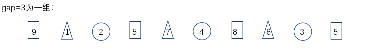
      2. After direct insertion sorting for each group
      3. 
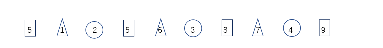
      4. In particular, for reverse order data, it is closer to order after pre scheduling.
2. Direct insert sort

• Single trip within a group

void ShellSort(int* a,int n){
     //Preprocessing data grouped by gap
     int gap=3;
     int end=0;
     int x=a[end+gap];
     while(end>=0){
         if(a[end]>x){
             a[end+gap]=a[end];
             end-=gap;
         }
         else break;
     }
     a[end+gap]=x;
}

void ShellSort(int* a,int n){
     //Preprocessing data grouped by gap     
     int gap=3;
     for(int i=0;i<n-gap;i+=gap){
         int end=i;
     	 int x=a[end+gap];
     	while(end>=0){
        	 if(a[end]>x){
            	 a[end+gap]=a[end];
             	end-=gap;
        	 }
         	else break;
     	}
     	a[end+gap]=x;
     }
}

• Promote to multiple groups

void ShellSort(int* a,int n){
     //Preprocessing data grouped by gap
     int gap=3;
     for(int j=0;j<gap;j++){
     	for(int i=j;i<n-gap;i+=gap){
         	int end=i;
     	    int x=a[end+gap];
     		while(end>=0){
        		 if(a[end]>x){
            	 	a[end+gap]=a[end];
             		end-=gap;
        	 	}
         		else break;
     		}
     		a[end+gap]=x;
     	}
     }
}

Time complexity: best O(N), worst F (n, gap) = (1 + 2 + 3... N/gap) * gap. The larger the gap, the faster the pre scheduling and the less close to the order. The smaller the gap, the slower the pre scheduling and the closer to order. Since it gradually becomes smaller and close to order, and the whole process is close to O(N), it can be estimated as NlogN from the following code. The official saying is O( N 1.3 {N^{1.3}} N1.3)

In fact, we can pre arrange multiple groups together, but each group is arranged in order.

void ShellSort(int *a,int n){
     //Preprocessing data grouped by gap
     int gap=3;
     //Many groups work together, one group at a time
     for(int i=0;i<n-gap;i++){
         	int end=i;
     	    int x=a[end+gap];
     		while(end>=0){
        		 if(a[end]>x){
            	 	a[end+gap]=a[end];
             		end-=gap;
        	 	}
         		else break;
     		}
     		a[end+gap]=x;
     	}
     }
}

At the same time, the pre sort is not only arranged once, but multiple pre sort (gap > 1) + direct insertion (gap==1).

Therefore, you can preprocess to gap=1 for many times. Each time / 2 can reach 1, but for example / 3 cannot reach 1. Therefore, if / 3 needs to be followed by + 1 every time.

void ShellSort(int *a,int n){
     //Preprocessing data grouped by gap
     int gap=n;
     while(gap>1){
     	//Many groups work together, one group at a time
        gap/=2;
        //gap=gap/3+1;
     	for(int i=0;i<n-gap;i++){
        	 	int end=i;
     	    	int x=a[end+gap];
     			while(end>=0){
        			 if(a[end]>x){
            	 		a[end+gap]=a[end];
             			end-=gap;
        	 		}
         			else break;
     			}
     			a[end+gap]=x;
     		}
     	}
	}
}

• Summary of Hill sort characteristics:

1. Hill sort is an optimization of direct insertion sort.
2. When gap > 1, the array is pre sorted. The purpose is to make the array closer to order. When gap == 1, the array is close to order, which will be very fast. In this way, the overall optimization effect can be achieved. After we implement it, we can compare the performance test.
3. The time complexity of Hill sort is not easy to calculate, because there are many gap value methods, which makes it difficult to calculate. Therefore, the time complexity of Hill sort given is not fixed O ( n 1.25 ) O(n^{1.25}) O(n1.25) or O ( 1.6 ∗ n 1.25 ) O(1.6*n^{1.25}) O(1.6∗n1.25)

2.2 select sort

2.2.1 direct selection sorting

Basic idea:

Each time, the smallest (or largest) element is selected from the data elements to be sorted and stored at the beginning of the sequence until all the data elements to be sorted are arranged.

Select sorting steps:

1. Select the data element with the largest (smallest) key in the element set array[i] – array[n-1]. If it is not the last (first) element in this group, it will be exchanged with the last (first) element in this group
2. In the remaining array[i] – array[n-2] (array[i+1] – array[n-1]) set, repeat the above steps until there is 1 element left in the set

For constant optimization, the maximum and minimum values are selected on the basis of selecting one at a time, but attention should be paid to the judgment of a special case.

• Write a single trip first

void SelectSort(int* a,int n){     
     int begin=0;int end=n-1;    
     while(begin<end){
     	int mini=begin,maxx=begin;
     	for(int i=begin;i<=end;i++){
        	 if(a[i]<a[maxx]) maxx=i;
        	 if(a[i]>a[mini]) mini=i;
     	}
         swap(&a[mini],&a[begin]);
     	 //maxx and begin are in the same position
         if(maxx==begin){
             maxx=mini;//Fix the position of maxx
         }
         swap(&a[maxx],&a[end]);
         begin++;end--;
     }
}

nature:

1. It is very easy to understand the direct selection sorting thinking, but the efficiency is not very good. It is rarely used in practice
2. Time complexity: O(N^2)
3. Space complexity: O(1)
4. Stability: unstable

Summary of characteristics of direct selection sorting:

1. It is very easy to understand the direct selection sorting thinking, but the efficiency is not very good. It is rarely used in practice
2. Time complexity: O(N^2)
3. Space complexity: O(1)
4. Stability: unstable

2.2.2 heap sorting

The upward adjustment heap building is O(N*logN). The downward adjustment is O (N).

void HeapSort(int* a,int n){
    //O(N)
    for(int i=(n-1-1)/2;i>=0;i--) adjustdown(a,n,i);
    int ed=n-1;
    //O(NlogN)
    while(ed>=0){
        swap(&a[0],&a[ed]);
        adjustdown(a,n-1,0);
        ed--;
    }
}

• Summary of characteristics of direct selection sorting:

1. Heap sorting uses heap to select numbers, which is much more efficient.
2. Time complexity: O(N*logN)
3. Space complexity: O(1)
4. Stability: unstable

2.3 exchange sorting

2.3.1 bubble sorting

void BubbleSort(int *a,int n){
  for(int i=0;i<n;i++){
   for(int j=0;j<n-i-1;j++){
       if(a[j]>a[j+1]) swap(&a[j],&a[j+1]);
   }  
  }
}

• Summary of bubble sorting characteristics:

1. Bubble sort is a sort that is very easy to understand
2. Time complexity: O(N^2)
3. Space complexity: O(1)
4. Stability: stable

2.3.2 quick sort

• hoare method

int Partion1(int* a, int left, int right)
{
	// Middle of three numbers -- in the face of the ordered worst case, the selected digits become the key and become the best case
	int mini = GetMidIndex(a, left, right);
	Swap(&a[mini], &a[left]);
	//Take the key on the left and go first on the right; on the contrary, take the key on the right and go first on the left. This is to ensure that the number that can be exchanged with keyi must be correct
	int keyi = left;
	while (left < right)
	{
		// Go first on the right and find the little girl
		while (left < right && a[right] >= a[keyi])
			--right;

		//Go left and find the big one
		while (left < right && a[left] <= a[keyi])
			++left;

		Swap(&a[left], &a[right]);
	}

	Swap(&a[left], &a[keyi]);

	return left;
}

• Excavation method

// Excavation method
int Partion2(int* a, int left, int right)
{
	// Middle of three numbers -- in the face of the ordered worst case, the selected digits become the key and become the best case
	int mini = GetMidIndex(a, left, right);
	Swap(&a[mini], &a[left]);

	int key = a[left];
	int pivot = left;
	while (left < right)
	{
		// Find a small one on the right and put it in the pit on the left
		while (left < right && a[right] >= key)
		{
			--right;
		}

		a[pivot] = a[right];
		pivot = right;

		// Find the big one on the left and put it in the pit on the right
		while (left < right && a[left] <= key)
		{
			++left;
		}
		a[pivot] = a[left];
		pivot = left;
	}

	a[pivot] = key;
	return pivot;
}

• Front and back pointer method

The idea of this method is to find a continuous sequence smaller than keyivalue through the front and back pointers.

cur find the small one and turn the small one to the left; prev pushes the large sequence to the right.

At the same time, single linked list / two-way linked list can also use this to sort. But the linked list can't get three numbers.

At the same time, there is an extreme case of fast platoon, that is, all data are the same or two data jump repeatedly. Fast platoon is strictly stuck O ( n 2 ) O(n^2) O(n2).

This method is not easy to get out of the boundary and easy to use. It is recommended to understand and remember this board.

int Partion3(int *a,int left,int right){
    int mini = GetMidIndex(a, left, right);
	Swap(&a[mini], &a[left]);
    int keyi=left;
    int prev=left;
    int cur=prev+1;
    while(cur<=right){
        if(a[cur]<a[keyi]&&++prev!=cur){
            swap(&a[cur],&a[prev]);
        }
        ++cur;
    }
    swap(&a[prev],&a[keyi]);
    return prev; 
}

void QuickSort(int *a,int left,int right){
    if(left>=right) return;
    int keyi=Partion3(a,left,right);
    QuickSort(a,left,keyi-1);
    QuickSort(a,keyi+1,right);
}

• Summary of quick sort features:

1. The overall comprehensive performance and usage scenarios of quick sort are relatively good, so we dare to call it quick sort
2. Time complexity: O(N*logN)
3. Space complexity: O(logN)
4. Stability: unstable

2.3.1 two optimizations of quick sort

• Select key by three numbers

int GetMidIndex(int* a, int left, int right)
{
	//int mid = (left + right) / 2;
	int mid = left + ((right - left) >> 1);
	if (a[left] < a[mid])
	{
		if (a[mid] < a[right])
		{
			return mid;
		}
		else if (a[left] > a[right])
		{
			return left;
		}
		else
		{
			return right;
		}
	}
	else // a[left] > a[mid]
	{
		if (a[mid] > a[right])
		{
			return mid;
		}
		else if (a[left] < a[right])
		{
			return left;
		}
		else
		{
			return right;
		}
	}
}

• When recursing to a small subinterval, you can consider using insertion sorting

int Partion3(int *a,int left,int right){
    int keyi=left;
    int prev=left;
    int cur=prev+1;
    while(cur<=right){
        if(a[cur]<a[keyi]&&++prev!=cur){
            swap(&a[cur],&a[prev]);
        }
        ++cur;
    }
    swap(&a[prev],&a[keyi]);
    return prev; 
}

Since the total number of layers of recursion between cells accounts for half of the layers of the whole recursion interval when reaching the deep layer of recursion, we reduce the number of recursion when recursing between cells. At this time, it is close to order, and the effect of direct insertion sorting is better.

void QuickSort(int *a,int left,int right){
    if(left>=right) return;
    //Inter cell optimization
    if(right-left+1<10){
        Insert(a+left,right-left+1);
    }
    else{
        int keyi=Partion3(a,left,right);
   	    QuickSort(a,left,keyi-1);
        QuickSort(a,keyi+1,right);
    }
}

2.3.2 non recursive version of fast scheduling

Sometimes the simple fast platoon is specially designed to explode the stack for you. And now the mainstream of the interview is non recursive simulation with stack.

The advantage here is that the heap is larger than the stack.

//For programs with too deep recursion, we can only consider non recursion.
void QuickSortNonR(int* a, int left, int right)
{
	Stack st;
	StackInit(&st);
	StackPush(&st, left);
	StackPush(&st, right);
	while (StackEmpty(&st) != 0)
	{
 		right = StackTop(&st);
 		StackPop(&st);
 		left = StackTop(&st);
 		StackPop(&st);
 		if(right - left <= 1)	continue;
 		int div = PartSort1(a, left, right);
 		// Take the reference value as the dividing point to form the left and right parts: [left, div) and [div+1, right)
 		StackPush(&st, div+1);
 		StackPush(&st, right);
 		StackPush(&st, left);
 		StackPush(&st, div);
	}
 	StackDestroy(&s);
}

2.4 merge sort

2.4.1 merge sort

Idea: suppose that the left side of the array is ordered and the right side is also ordered, and O (N) is merged into an ordered array. At the same time, it is necessary to use a third-party array. That is to say, merging sorting consumes space complexity.

10 6 7 1 3 9 4 2
1 6 7 10 	2 3 4 9
tmp:1 2 3 4 6 7 9 10

The premise of this method is that the left interval is orderly and the right interval is also orderly. Just like fast scheduling, smaller intervals are processed.

void _MergeSort(int* a,int left,int right,int* tmp){
    if(left>=right) return;
 	int mid=(left+right)/2;
     //If [left,mid] is ordered and [mid+1,right] is ordered, it can be ordered
	_MergeSort(a,left,mid,tmp);
    _MergeSort(a,mid+1,right,tmp);
    
    int begin1=left,end1=mid;
    int begin2=mid+1,end2=right;
    int idx=left;
    while(begin1<=end1&&begin2<=end2){
        if(a[begin1]<a[begin2]) tmp[idx++]=a[begin1++];
        else tmp[idx++]=a[begin2++];
    }
    while(begin1<=end1){
        tmp[idx++]=a[begin1++];
    }
    while(begin2<=end2){
        tmp[idx++]=a[begin2++];
    }
    //Copy tmp array back to a
    for(int i=left;i<=right;i++) a[i]=tmp[i];
}
void MergeSort(int *a ,int n){
    int * tmp=(int*)malloc(n*sizeof(int));
    if(tmp==NULL){
        perror("malloc fail\n");exit(-1);
    }
    _MergeSort(a,0,n-1,tmp); 
    free(tmp);
    tmp=NULL; 
}

• Summary of characteristics of merge sort:

1. The disadvantage of merging is that it requires O(N) space complexity. The thinking of merging sorting is more to solve the problem of external sorting in the disk.
2. Time complexity: O(N*logN)
3. Space complexity: O(N)
4. Stability: stable

2.4.2 non recursive merge sort

Non recursive can be handled by using queue bfs, but stack simulation is the same process as dfs.

Consider the single trip method, first consider the interval of one-to-one element merging, and then increase the interval distance.

void MergeSortNonR(int *a,int n){
     int *tmp=(int*)malloc(n*sizeof(int));
     if(tmp==NULL){
         printf("Error!\n");
         exit(-1);
    }
     int gap=1;
     while(gap<n){
     	for(int i=0;i<n;i+=2*gap){
         	//[i,i+gap-1],[i+gap,i+2*gap-1]
            int begin1=i;int end1=i+gap-1;
            int begin2=i+gap;int end2=i+2*gap-1;
            int idx=i;
            while(begin1<=end1&&begin2<=end2){
                if(a[begin1]<a[begin2]){
                    tmp[idx++]=a[begin1++];
                }else tmp[idx++]=a[begin2++];
            }
            while(begin1<end1){
                tmp[idx++]=a[begin1++];
            }
            while(begin2<end2){
                tmp[idx++]=a[begin2++];
            }
     	}
        for(int i=0;i<n:i++){
            a[i]=tmp[i];
        }
        gap*=2;
     }
}

But the above code is only right 2 i 2{^i} 2i length data holds. Non recursive versions should consider boundaries.

Boundary crossing:

1. [begin1, end1], [begin2, end2]. End1, begin2, end2 are out of bounds.
2. [begin1, end1], [begin2, end2]. Begin2, end2 are out of bounds.
3. [begin1, end1], [begin2, end2]. End2 is out of bounds.

void MergeSortNonR(int *a,int n){
     int *tmp=(int*)malloc(n*sizeof(int));
     if(tmp==NULL){
         printf("Error!\n");
         exit(-1);
    }
     int gap=1;
     while(gap<n){
     	for(int i=0;i<n;i+=2*gap){
         	//[i,i+gap-1],[i+gap,i+2*gap-1]
            int begin1=i;int end1=i+gap-1;
            int begin2=i+gap;int end2=i+2*gap-1;
            //end1 is out of bounds, begin2 and end2 do not exist
            if(end1>=n){
                end1=n-1;
            }
            if(begin2>=n){
                begin2=n; end2=n-1;///It should be corrected to a non-existent interval, otherwise there will be two visits [8,8] [8,8] that will lead to the index subscript crossing the boundary.
            }
            if(end2>=n){
                end2=n-1;
            }
            int idx=i;
            while(begin1<=end1&&begin2<=end2){
                if(a[begin1]<a[begin2]){
                    tmp[idx++]=a[begin1++];
                }else tmp[idx++]=a[begin2++];
            }
            while(begin1<=end1){
                tmp[idx++]=a[begin1++];
            }
            while(begin2<=end2){
                tmp[idx++]=a[begin2++];
            }
     	}
        for(int i=0;i<n:i++){
            a[i]=tmp[i];
        }
        gap*=2;
     }
     free(tmp);
     tmp=NULL;
}

Due to the unified processing of the above code, there are some boundaries to consider when putting back the original array. We can go back like recursion.

void MergeSortNonR(int *a,int n){
     int *tmp=(int*)malloc(n*sizeof(int));
     if(tmp==NULL){
         printf("Error!\n");
         exit(-1);
    }
     int gap=1;
     while(gap<n){
     	for(int i=0;i<n;i+=2*gap){
         	//[i,i+gap-1],[i+gap,i+2*gap-1]
            int begin1=i;int end1=i+gap-1;
            int begin2=i+gap;int end2=i+2*gap-1;
            //end1 out of bounds | begin2 > = n, the original array can be used directly without merging.
            if(end1>=n||begin2>=n){
                break;
            }
            //End2 is out of bounds and needs to be merged. Correct end2
            if(end2>=n){
                end2=n-1;
            }
            int idx=i;
            while(begin1<=end1&&begin2<=end2){
                if(a[begin1]<a[begin2]){
                    tmp[idx++]=a[begin1++];
                }else tmp[idx++]=a[begin2++];
            }
            while(begin1<=end1){
                tmp[idx++]=a[begin1++];
            }
            while(begin2<=end2){
                tmp[idx++]=a[begin2++];
            }
            for(int j=i;j<=end2:j++){
            	a[j]=tmp[j];
        	}
     	}
        gap*=2;
     }
     free(tmp);
     tmp=NULL;
}

2.5 non comparative sorting

2.5.1 counting and sorting

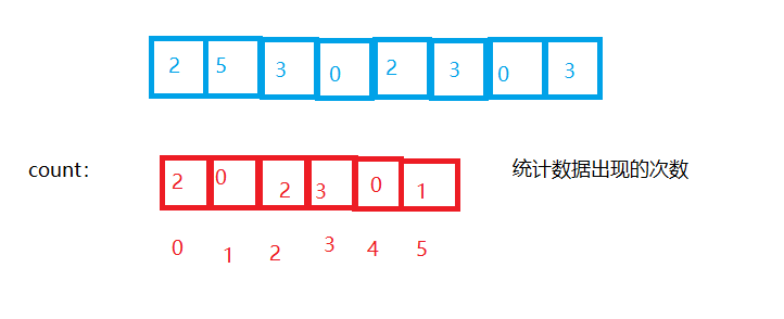
Idea: counting sorting, also known as pigeon nest principle, is a deformation application of hash direct addressing method.

Operation steps:

1. Count the number of occurrences of the same element O (N)
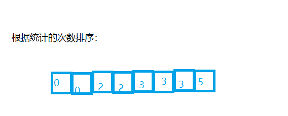
2. According to the statistical results, the sequence is recovered into the original sequence O (range)

Or the complexity is O (max (N, range))

But for example, the data is: 10001200101150013001301. Do you want to open 1501 sizes? We can simply optimize to open MAX-MIN+1 space.

Mapping position: x-min

Relative mapping.

It can be seen that counting sorting is more suitable for the situation of relatively tight data.

void CountSort(int* a,int n){
    int max=a[0],min=a[0];
    for(int i=0;i<n;i++){
		if(a[i]>max) max=a[i];
         if(a[i]<min) min=a[i];
    }
    int range=max-min+1;
    int* count=(int*)malloc(range*sizeof(int));
    memset(count,0,sizeof(int)*range);
    if(count==NULL) perror("malloc error\n");
    //Statistical times
    for(int i=0;i<n;i++){
        count[a[i]-min]++;
    }
    //Sort by number of times
    int idx=0;
    for(int i=0;i<range;i++){
	    while(count[i]--){
            a[idx++]=i+min;
        }
    }
}

For negative numbers, you can use unsigned to turn them into positive numbers, but the time complexity explodes.

• Summary of characteristics of count sorting

1. Counting sorting is very efficient when it is in the data range set, but its scope of application and scenarios are limited. If the range is large, floating-point numbers are not suitable.

2. Time complexity: O(MAX(N, range))

3. Space complexity: O (range)

4. Stability: stable

3. Sorting summary

O ( N 2 ) O(N^{2}) O(N2): direct insert, select sort, bubble sort.

O ( N ∗ l o g ( N ) ) O(N*log(N)) O(N * log(N)): Hill sort, heap sort, quick sort, merge sort.

In the interview, it is easiest to write fast, merge and pile up.

Stability: it is assumed that there are multiple records with the same keyword in the record sequence to be sorted. If sorted, the relative order of these records remains unchanged, that is, in the original sequence, r[i]=r[j], and r[i] is before r[j], while in the sorted sequence, r[i] is still in r[j] Previously, it was said that this sorting algorithm was stable; otherwise, it was called unstable. - whether the relative position of the same value in the array changes after sorting may be unstable. If it can be guaranteed to remain unchanged, it is stable.

What is the meaning of stability? For example, if there is a structure data, for the first dimension with the same value, you can see the second dimension.

First, all sorts can be unstable. Let's see which sorts can be stable after control.

Sorting method	stability	reason
Direct insert sort	stable	You can control not to allow the exchange of the same value
Shell Sort	instable	Assignment of the same value to a group cannot be guaranteed
Select sort	instable	5 , 4 , 1 , 5 , 0 , 9 {5,4,1,5,0,9} 5,4,1,5,0,9 will swap the first 5 to the back, resulting in instability
Heap sort	instable	5 , 5 , 5 , 2 , 4 {5,5,5,2,4} When 5,5,5,2,4 is adjusted, it becomes 4 , 5 , 5 , 2 , 5 {4,5,5,2,5} 4,5,5,2,5 the first 5 to the last position
Bubble sorting	stable	Equal no exchange
Quick sort	instable	5....5...5 {5....5...5} 5.... 5... 5 fast row. Find strictly large numbers on the left and strictly small numbers on the right. The first 5 will reach some positions in the middle. Then the recursive interval will not change the current position
Merge sort	stable	1 , 2 , 2 , 4 {1,2,2,4} 1,2,2,4 and 1 , 2 , 3 {1,2,3} 1, 2, 3. When equal, the one on the left comes first.
Count sort	instable	After counting, the numbers are different

1. Quick sort algorithm is a sort algorithm based on ().
	A Divide and conquer
	B Greedy 
	C Recursive method
	D Dynamic programming method
2.To record (54),38,96,23,15,72,60,45,83)When performing a direct insertion sort from small to large, when the eighth record 45 is inserted into the order
 In order to find the insertion position, the table needs to be compared () times? (compare from back to front)
	A 3
	B 4
	C 5
	D 6
3.Occupied in the following sorting methods O(n)The of secondary storage space is
	A Simple sort
	B Quick sort
    C Heap sort
	D Merge sort
4.The following sorting algorithms are stable and have a time complexity of O(n2)Yes ()
	A Quick sort
	B Bubble sorting
	C Direct selection sort
	D Merge sort
5.About sorting, the following statement is incorrect
	A The fast scheduling time complexity is O(N*logN)，Space complexity is O(logN)
	B Merge sort is a stable sort,Heap sorting and fast scheduling are unstable
	C When the sequence is basically ordered, the fast sorting degenerates into bubble sorting, and the direct insertion sorting is the fastest
	D Merge sort space complexity is O(N), The complexity of heap sort space is O(logN)
6.Among the following ranking methods, the least time complexity in the worst case is ()
	A Heap sort
	B Quick sort
	C Shell Sort 
	D Bubble sorting
7.Set a set of initial record keyword sequence as(65,56,72,99,86,25,34,66)，The first keyword 65 is used as the benchmark
 The quick sort result is ()
	A 34，56，25，65，86，99，72，66
	B 25，34，56，65，99，86，72，66
	C 34，56，25，65，66，99，86，72
	D 34，56，25，65，99，86，72，66

answer:
1.A
2.C
3.D
4.B
5.D
6.A
7.A