catalogue
Today's goal:
Draw an image and title it
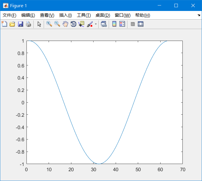
First, let's draw a very simple figure, for example, draw an image of y = cos x.
The code is as follows:
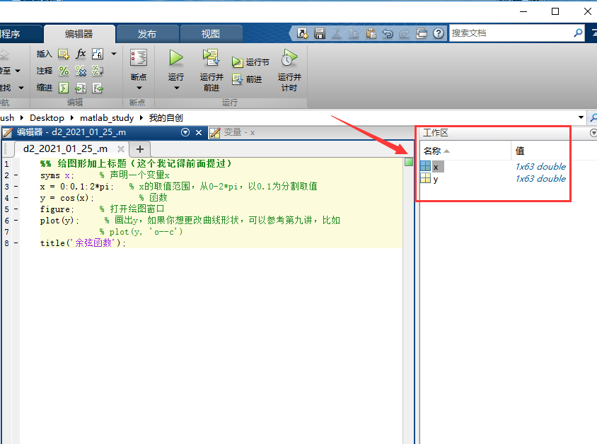
%% Add a title to the graphic (I remember mentioning this earlier)

syms x; % Declare a variable x

x = 0:0.1:2*pi; % x Value range of, from 0-2*pi,With 0.1 It is a split value

y = cos(x); % function

figure; % Open the drawing window

plot(y); % Draw y,If you want to change the shape of the curve, you can refer to Lecture 10, for example

% plot(y, 'o--c')
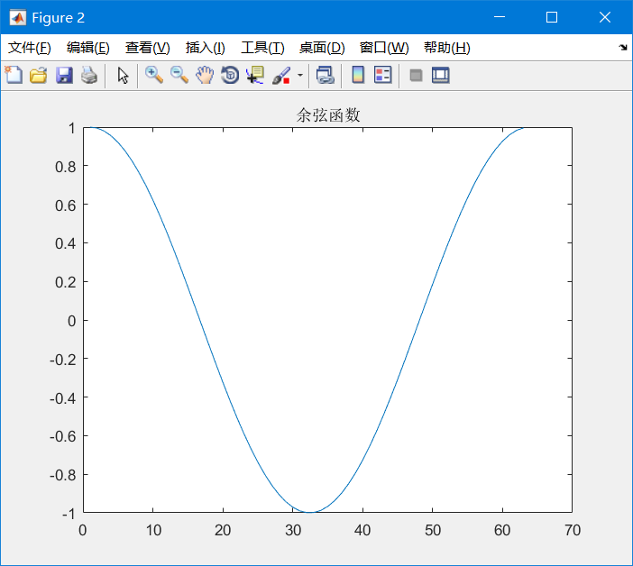
If we want to add a title to this figure, we just need to use title() You can:
The code is as follows:
%% Add a title to the graphic (I remember mentioning this earlier)

syms x; % Declare a variable x

x = 0:0.1:2*pi; % x Value range of, from 0-2*pi,With 0.1 It is a split value

y = cos(x); % function

figure; % Open the drawing window

plot(y); % Draw y,If you want to change the shape of the curve, you can refer to Lecture 10, for example

% plot(y, 'o--c')

title('cosine function');
At first glance, this code is very common, it seems ordinary, but please look at the part of plot carefully!!!!
Some students may vaguely remember that I used it ploy(x, y) To draw a picture, but today I only use it plot(y) The picture came out, you can refer to the front Lecture 10:
Why? If everyone can think about it carefully, I believe everyone can find the problem.
Additional knowledge: this hand tool can drag images (the coordinate axis will also change)
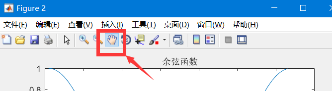
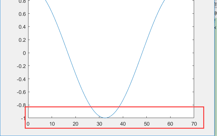
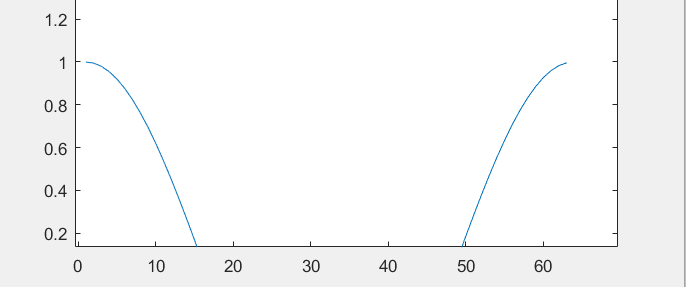
There is a big problem with the above image: please look at the abscissa bar of the image, as shown in the following figure (the latter figure is the picture when the first point is dragged close to the abscissa axis with a hand tool):
Or we can use this tool (the scientific name is data cursor) to view the value of this point:
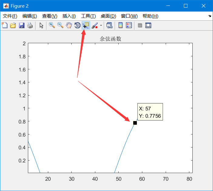
EH ~ no, why is the coordinate axis 1-63? Isn't my value range of x 0-2*pi?
EH ~ how do you know it's 63 instead of 64?
Let's look at this axis, 60 +, what can we think of?
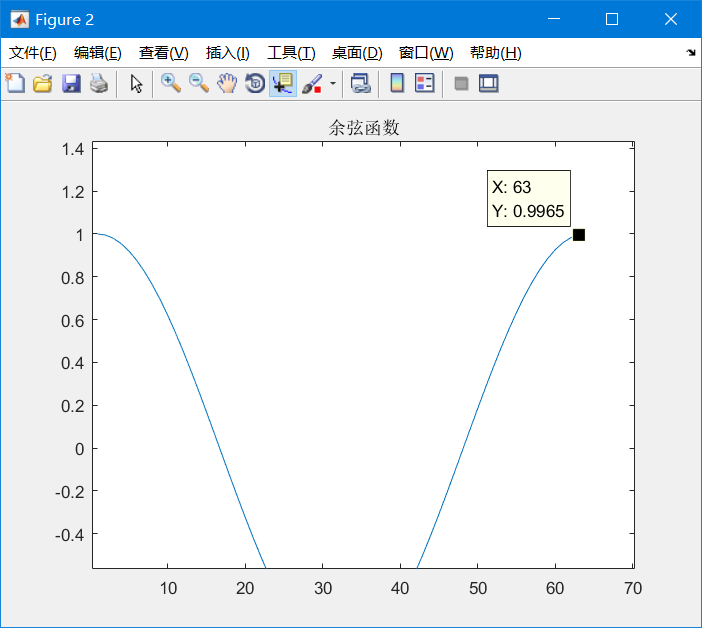
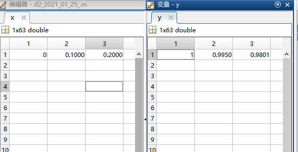
Yes, our definition of X is as follows: x = 0:0.1:2*pi, that is, X looks continuous but actually discontinuous (as mentioned earlier). In fact, the value of X is a matrix, in which 0.1, 0.2... Up to 2*pi. 2*pi is a little more than 6.28, so it stops at 6.2 at most. Therefore, the value of X is actually the 63 data, and y = cos x is actually the value of COS calculated relative to the value of each X. therefore, when x = 0, y = cosx = > y = 1, and so on, we can see the real value of X and Y in the workspace:
In this way, we can know the function of plot.
Plot drawing, if there is only one parameter, the abscissa is 1, 2, 3.... By analogy, the parameter is taken as the abscissa as 1, 2, 3.. For plot(y), we can see that when the abscissa is 1, the ordinate takes 1 (y = 1), and when the abscissa is 2, the ordinate takes 0.9950 (y = 0.9950).... and so on.
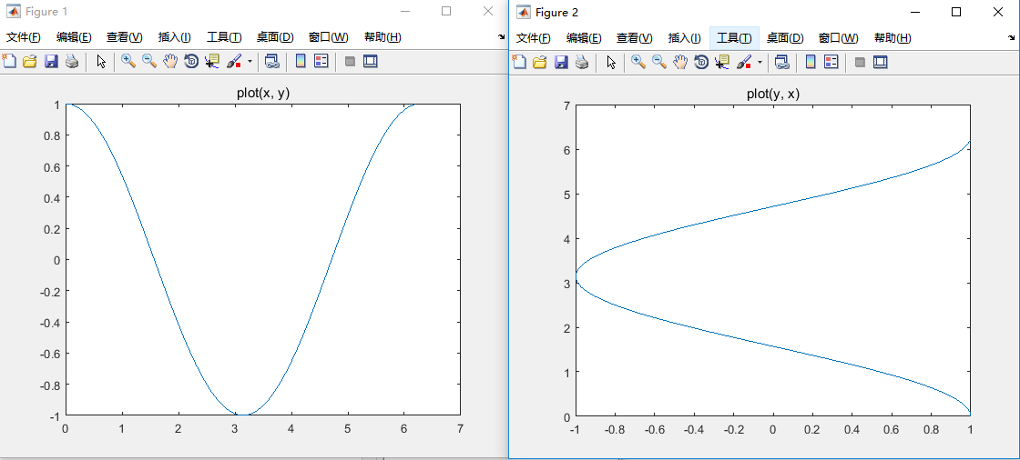
If there are two parameters, the first parameter is the abscissa and the second is the ordinate. The amount of values in the two parameters should be the same, so that the corresponding drawing can be made. For example, we use plot(x,y) and plot(y, x):
The code is as follows:
%% Add a title to the graphic (I remember mentioning this earlier)

syms x; % Declare a variable x

x = 0:0.1:2*pi; % x Value range of, from 0-2*pi,With 0.1 It is a split value

y = cos(x); % function

figure; % Open the drawing window

plot(x, y); % Draw y,If you want to change the shape of the curve, you can refer to Lecture 9, for example

% plot(y, 'o--c')

title('plot(x, y)');

figure

plot(y, x);

title('plot(y, x)');
Additional thought: what if the parameters of plot are three?
If you really write the following code at this time:
%% plot There are three parameters

clear all;

syms x;

x = 0:0.1:2*pi;

y = sin(x);

z = cos(x);

figure;

plot(x, y, z);
Then, no accident, your matlab should flash back.
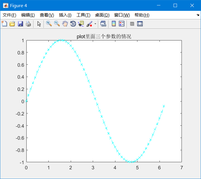
Remember that we said that plot() can set the point shape, curve style and color of the function curve. In fact, the third parameter needs to be a string (such as' x--c '):
The code is as follows:
%% plot There are three parameters
clear all;
syms x;
x = 0:0.1:2*pi;
y = sin(x);
figure;
plot(x, y, 'x--c');
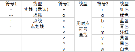
title('plot There are three parameters');The shape setting of the third parameter was mentioned earlier, and I'll copy the picture here (don't forget that the three symbols don't distinguish the sequence. There is also the propertyname parameter, which is actually useless. Just mention it here. We should know that the following table should be enough for drawing, so we won't talk about it here.)
So, I believe you can deeply understand the role of plot().
Subgraph drawing
subplot() can be used to divide a figure into multiple blocks. This is a very simple function. See the code:
%% Subgraph drawing
x = 0:0.1:2*pi; % Set variable range
y = sin(x); % First function
z = cos(x); % Second function
figure; % Create an image palette
subplot(3, 2, 1); % Divide the drawing board into 3 rows and 2 columns, and select the first area
plot(x, y); % Draw a picture in this area
title('y = sin x'); % The name of this area
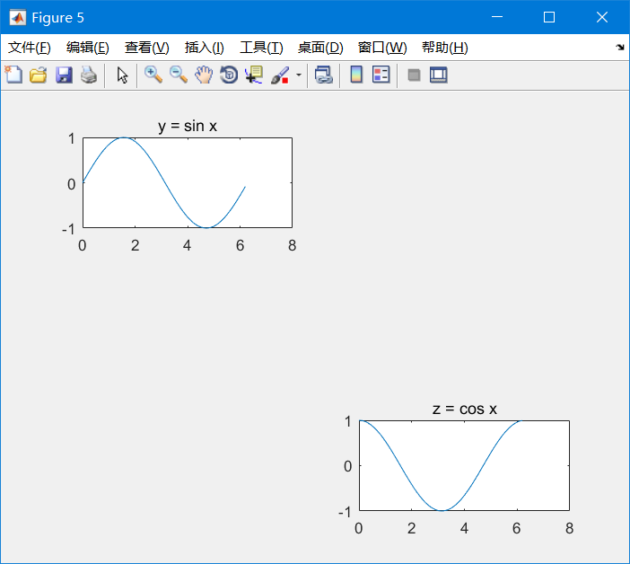
subplot(3, 2, 6); % Divide the drawing petals into 3 rows and 2 columns, and select the sixth area
plot(x, z); % draw z = cosx
title('z = cos x'); % nameThe last image appears as follows:
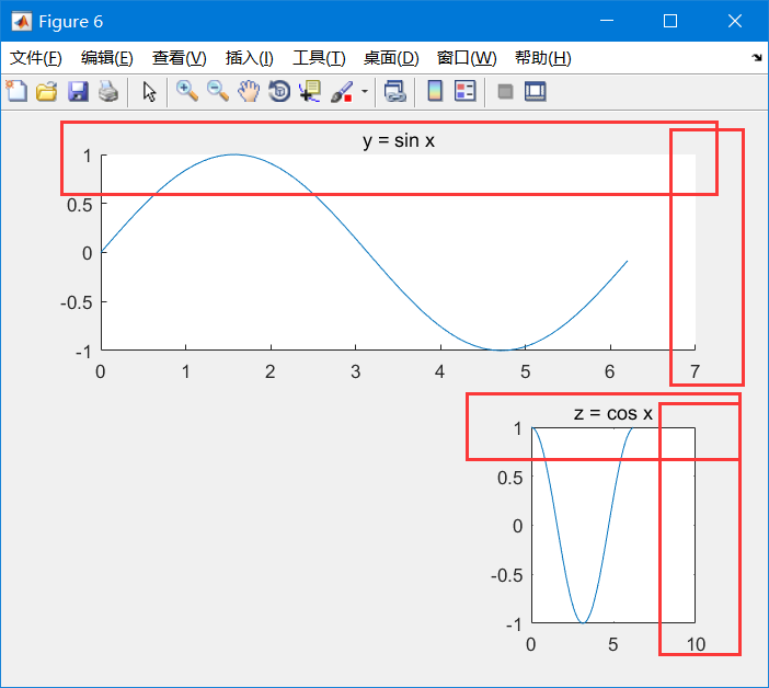
Extra thought: if I want to draw two pictures, and their partition methods are different? Can we draw different drawings with different shapes of the divided areas and select the non overlapping parts? Let's have a try!
%% Subgraph drawing
x = 0:0.1:2*pi; % Set variable range
y = sin(x); % First function
z = cos(x); % Second function
figure; % Create an image palette
subplot(2, 1, 1); % Divide the drawing board into two rows and one column. Select the first area, which is actually the first row
plot(x, y); % Draw a picture in this area
title('y = sin x'); % The name of this area
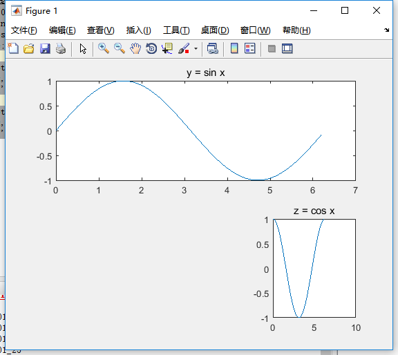
subplot(2, 3, 6); % Divide the drawing petals into 2 rows and 3 columns, and select the sixth area
plot(x, z); % draw z = cosx
title('z = cos x'); % nameThe following are the output results, which seem to meet our expectations:
Therefore, when we divide the region, we can divide it flexibly according to the needs of the image. This subplot is only a logical division of the region, not a real division of the region!!!!
Some little knowledge
grid setting border
grid on turns on the border, which is off by default (grid off)
The code is as follows:
%% Subgraph drawing
x = 0:0.1:2*pi; % Set variable range
y = sin(x); % First function
z = cos(x); % Second function
figure; % Create an image palette
subplot(2, 1, 1); % Divide the drawing board into 3 rows and 2 columns, and select the first area
plot(x, y); % Draw a picture in this area
title('y = sin x'); % The name of this area
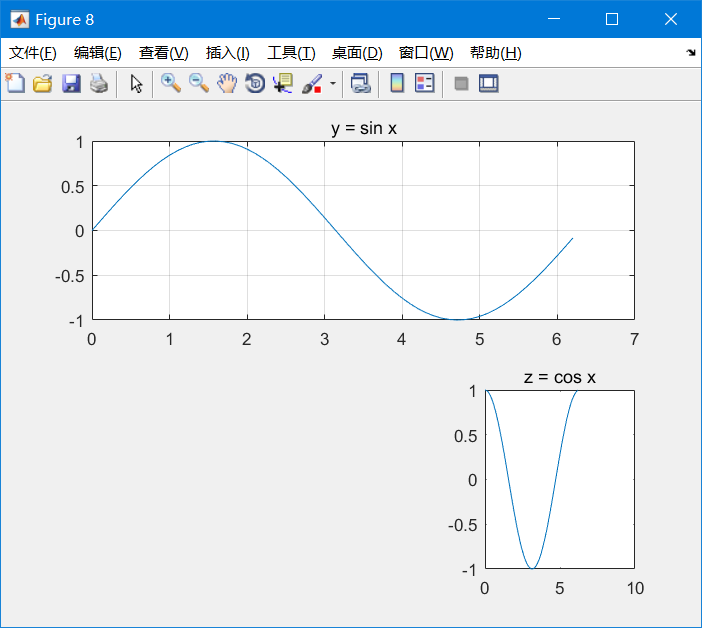
grid on; % Frame this area
subplot(2, 3, 6); % Divide the drawing petals into 2 rows and 3 columns, and select the sixth area
plot(x, z); % draw z = cosx
title('z = cos x'); % name
box set border
box off closes the border of the image. This is on by default (box on). In fact, I don't think it's useful. It's mainly for the convenience of observation at the critical point
The code is as follows:
%% Subgraph drawing

x = 0:0.1:2*pi; % Set variable range

y = sin(x); % First function

z = cos(x); % Second function

figure; % Create an image palette


subplot(2, 1, 1); % Divide the drawing board into 3 rows and 2 columns, and select the first area

plot(x, y); % Draw a picture in this area

title('y = sin x'); % The name of this area

box off; % Set border off for this area


subplot(2, 3, 6); % Divide the drawing petals into 2 rows and 3 columns, and select the sixth area

plot(x, z); % draw z = cosx

title('z = cos x'); % name
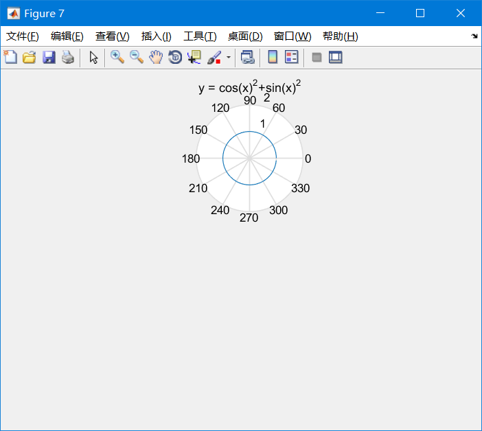
Polar plot
Some images only have polar coordinates, which are difficult to solve or do not have rectangular coordinates, so the polar coordinate system needs to be used. The polar drawing parameters are almost the same as Plot(). Take an example:
The code is as follows:
%% polar()

x = 0:0.1:2*pi; % Set variable range

y = cos(x).^2+sin(x).^2;

% The first function, in matlab In,^ Represents power, not XOR.

% however matlab Are matrices, so you need to add one before the operator . ,Indicates that all elements in the matrix are squared

% We all know, z It's the polar representation of a circle.

figure; % Create an image palette

subplot(2, 1, 1); % Divide the drawing petals into 2 rows and 1 column, and select the first area

polar(x, y); % draw y = cosx

title('y = cos(x)^2+sin(x)^2'); % name

% The partition is to tell you, polar()It can also operate in partitions
Today's summary
Today I learned the following:
- How exactly do plot() and plot() work
- Use of some small tools in matlab, such as data cursor
- Draw polar coordinates
- Draw subgraph
- Some small functions