1, Neural network applied to classification problem: suppose there are m training samples, each containing a set of input x and a set of output y, l represents the number of neural network layers, SlS_{l}Sl represents the number of neurons in layer L. There are two kinds of neural network classification problems
(1) Binary classification: y can only be 0 or 1, with only one output unit.
(2) Multi category classification: there are K different classes, K output units, assuming that the output K-dimensional vector, yi=1y_{i}=1yi = 1 means to be classified into class I.
The cost function of regularization of multi class classification is: J (θ) = - 1m [∑ i=1m ∑ k = 1K YK (I) log (H θ (x(i)))k+(1 − yk(i))log(1 − (H θ (x (I))) k] + λ 2m ∑ l=1L − 1 ∑ i=1Sl ∑ j=1Sl+1(Θ Ji (L)) 2J \ left (\ theta \ right) = - \ frac {1} {m} [\ sum_ {i=1}^{m}\sum_ {k=1}^{k}y_ {k}^{\left ( i \right )}log\left ( h_ {\theta }\left ( x^{\left ( i \right )} \right ) \right )_ {k}+\left ( 1-y_ {k}^{\left ( i \right )} \right )log\left ( 1-\left ( h_ {\theta } \left ( x^{\left ( i \right )} \right )\right ) _ {k}\right )]+\frac{\lambda }{2m}\sum_ {l=1}^{L-1}\sum_ {i=1}^{S_ {l}}\sum_ {j=1}^{S_ {l+1}}\left ( \Theta_ {ji}^{\left ( l \right )}\right )^{2}J(θ)=−m1​[i=1∑m​k=1∑k​yk(i)​log(hθ​(x(i)))k​+(1−yk(i)​)log(1−(hθ​(x(i)))k​)]+2mλ​l=1∑L−1​i=1∑Sl​​j=1∑Sl+1​​(Θji(l)​)2
Where h θ (x) ∈ RKh_{\theta }\left ( x \right )\in R^{K}hθ​(x)∈RK，(hθ(x))i=ithoutput\left ( h_{\theta }\left ( x \right )\right )_{i}=i^{th}output(hθ​(x))i​=ithoutput.
The term of regularization is to exclude every layer of θ 0 \ theta_ After {0} θ 0, the sum of theta matrices of each layer. The innermost j loop loops all rows (by SL + 1s_ The number of active units in the layer {L + 1} SL + 1 is determined by the number of active units in the layer {L + 1} SL + 1). Cycle I cycles all columns (by the layer, i.e. SLS_ {l} The number of active units of the SL layer is determined).
When performing gradient descent method or advanced optimization algorithm, it is necessary to select some initial values for the variable θ. For logic regression, all parameters can be initialized to 0, but the neural network is not feasible, which will cause all the activation units in the second layer to be the same value. The idea of random initialization can be used to initialize the weight randomly to a number close to 0, ranging from - ε to ε.
2, Back propagation algorithm
This algorithm is used to calculate the partial derivative ∂ θ ij(l)J(θ) of the cost function ∂ frac {\ partial} {\ partial \ theta_ {ij} ^ {\ left (L \ right)}} J \ left (\ theta \ right) ∂ θ ij(l) ∂ J(θ), first calculate the error of the last layer, and then calculate the error of each layer in reverse until the last layer. Suppose that the neural network is of the following four layers structure: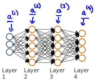

Starting from the error of the last la y er, use δ j(l) Delta_ {j} {\ left (3 \ right)} \ right) ^ {t} \ delta ^ {\ left (4 \right )}*g^{'}\left ( z^{\left ( 3 \right )} \right )δ(3)=(θ(3))Tδ(4)∗g′(z(3))
So suppose λ = 0, that is, when no regularization is done: ∂ θ ij(l)J(θ) = AJ (L) δ IL + 1 \ frac {\ partial} {\ partial \ theta_ {ij}^{\left ( l \right )}}J\left ( \theta \right )=a_ {j}^{\left ( l \right )}\delta _ {i}^{l+1}∂θij(l)​∂​J(θ)=aj(l)​δil+1​
Where l represents the current calculated layer, j represents the subscript of the active unit in the current calculation layer, and i represents the subscript of the error unit in the next layer.
When the training set is a characteristic matrix and the error unit is a matrix, use Δ ij(l) Delta_ {I j} ^ {\ left (l \ right)} Δ ij(l) is used to represent the error matrix, that is, the error caused by the influence of the j-th parameter on the i-th activation unit of the l-th layer. The algorithm is expressed as: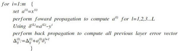

3, Gradient test
When using gradient descent algorithm for more complex models such as neural network, there may be some imperceptible errors. Although the cost seems to be decreasing, the final result may not be the optimal solution. Therefore, a Numerical Gradient Checking method is adopted to check whether the calculated derivative value is correct by estimating the gradient value.
The method is to select two very close points along the tangent direction in the cost function and calculate the average value of the two points to estimate the gradient. That is to say, for a specific θ, calculate the substitute value at θ - ɛ and θ + ɛ (ɛ is a very small value, usually 0.001), and then calculate the average of the two costs to estimate the substitute value at θ.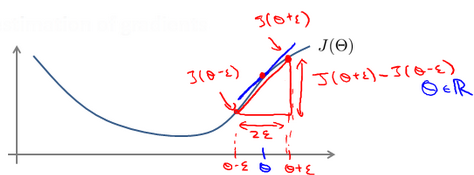

4, Steps of neural network
The first thing is to choose the network structure, that is, to decide how many layers to choose and how many cells each layer has. The number of units in the first layer is the number of features in the training set, and the number of units in the last layer is the number of classes in the result. When the number of hidden layers is greater than 1, it is better to have the same number of cells in each hidden layer. In general, the more units in the hidden layer, the better. The number of units in each hidden layer should match the number of features, which can be the same as the number of input features, or twice or three or four times of it. The specific steps of training neural network are as follows:
1. Random initialization of parameters
2. Using the forward propagation method to calculate all h θ (x)
3. Write the code to calculate the cost function J
4. Calculation of all partial derivatives by back propagation method
5. Using numerical test method to test these partial derivatives
6. Use optimization algorithm to minimize cost function
5, Based on the practice materials of Wu Enda's machine learning course, the neural network is trained to carry out multi category classification, and the background is to recognize handwritten numbers. In the previous paper, the trained parameters are directly used to construct neural network for classification, and now the task includes learning the parameters of neural network using back propagation algorithm. Write related functions to build neural network from scratch. For code implementation, please refer to: Python implementation of Wu Enda's machine learning task (4): neural network (back propagation) . However, after trying to implement it, because of the limitation of conditions, it can not run on my computer, and the running speed is too slow, so I try to use the pytorch framework to implement it. Code implementation source reference: Neural Networks Learning
The original training data set is saved in matlab data storage format. mat. There are 5000 training samples in the data. Each training sample is a number of 20 pixels × 20 pixels gray image. Each pixel is represented by a floating-point number, which represents the gray intensity of the location. Each grid of 20 × 20 pixels is expanded into a vector of 400 dimensions to obtain a 5000 × 400 matrix X, and each row is taken as a training sample. The second part of the training set is the 5000 dimensional vector y representing the label of the training set, "0" is marked as "10", and "1" to "9" are marked as "1" to "9" in natural order.
The related function implementation code is as follows:

import torch
import torch.nn as nn
import torch.utils.data as Data
from scipy.io import loadmat
import matplotlib.pyplot as plt

#Define neural network model
class NeuralNetwork(nn.Module): #inherit nn.Module class
  def __init__(self):
    super(NeuralNetwork,self).__init__()  #Call the constructor of the parent Module
    self.linear1=nn.Linear(400,25)  #Set hidden layer and define input and output dimensions
    self.sigmoid=nn.Sigmoid() #Introduce Sigmoid function
    self.linear2=nn.Linear(25,10) #Set output layer

  def forward(self,X):  #Forward propagation function
    X=self.linear1(X)
    X=self.sigmoid(X) 
    X=self.linear2(X) 
    out=self.sigmoid(X) 
    return out

#Initialize parameters with uniform distribution
def InitParameters(net,epsilon_init):
  for m in net.modules():
    if isinstance(m,nn.Linear):
      weight_shape=m.weight.data.shape
      bias_shape=m.bias.data.shape
      m.weight.data=torch.rand(weight_shape)*2*epsilon_init-epsilon_init  #The range of random initialization parameters is [- epsilon_init,epsilon_init]
      m.bias.data=torch.rand(bias_shape)*2*epsilon_init-epsilon_init

#Regularization
def add_regular_item(net,m,lm):
  for module in net.modules():
    if isinstance(module,nn.Linear):
      module.weight.grad.data.add_(lm/m*module.weight.data) #Add gradient regularization term λ θ / m

#Training model
def train(net,num_epochs,train_iter,loss,optim,lm,print_frequence):
  for epoch in range(num_epochs):
    n_batch,sum_loss,m=0,0.0,0
    for X,y in train_iter:
      optim.zero_grad() #Set the gradient to zero, that is, change the derivative of loss with respect to weight to 0
      m=y.shape[0]
      y_hat=net(X)  #Forward propagation to find the predicted value
      l=loss(y_hat,y.view(-1,y.shape[1])).sum() #Calculate loss
      l.backward()  #Back propagation gradient
      add_regular_item(net,m,lm)  #Regularization
      optim.step()  #Update all parameters
      sum_loss+=l
      n_batch+=1
    if print_frequence>0:
      if (epoch+1)%print_frequence==0:
        print("epoch:%d,average loss:%f"%(epoch+1,sum_loss/n_batch))
        print("epoch:%d,train accuracy:%0.2f%%\n"%(epoch+1,evaluate(net,train_iter)))

#Calculation accuracy
def evaluate(net,test_iter):
  sum_accurate,num_data=0.0,0
  for X,y in test_iter:
    y=y.view(-1,y.shape[1]) #Get actual value
    num_data+=y.shape[0] #Total number of samples
    y_hat=net(X)  #Get forecast
    sum_accurate+=(y_hat.argmax(1)==y.argmax(1)).sum()  #Get the right number of predictions
  return 100*sum_accurate.float()/num_data

The code of data loading, initialization and training neural network is as follows:

train_file_data=loadmat('multi_class_cl.mat') #Reading data set in matlab format
X=torch.tensor(train_file_data['X'],dtype=torch.float) #Get feature data and generate corresponding torch.FloatTensor
y=torch.tensor(train_file_data['y'],dtype=torch.long)-1  #Obtain classification data and generate corresponding torch.LongTensor , classify the category data from 0. Originally, 1-9 is category 1-9, 10 is category 0, 0-8 is category 1-9, and 9 is category 0
y=torch.zeros(y.shape[0],max(y)+1).scatter_(dim=1,index=y,value=1)  #Each category in y is transformed into a vector, and the corresponding category is set to 1 at the corresponding position of the vector
#print(X.shape)
#print(y.shape)

#Define the necessary variables and train the network
net=NeuralNetwork() #Define neural network model
batch_size,num_epochs,print_frequency,lr,lm=250,1200,50,0.5,0 #batch_size is the number of samples to be processed before updating internal model parameters, num_epochs defines the number of times the learning algorithm works in the whole training data set. lm is the regularization parameter
loss=nn.BCELoss() #Define loss function
InitParameters(net,0.12)  #Initialization parameters
optim=torch.optim.SGD(net.parameters(),lr)  #Using SGD optimization method to construct optimizer, lr is learning rate
train_dataset=Data.TensorDataset(X,y) #Load data
train_iter=Data.DataLoader(train_dataset,batch_size=batch_size,shuffle=True)  #The data loader divides the training data into several groups and draws out the batch each time_ Size samples, shuffle. At the beginning of each epoch, the data will be scrambled again
train(net,num_epochs,train_iter,loss,optim,lm,print_frequency)  #Training model

When batch_size=250，num_ When epochs = 1200, lm=0, run the model code twice with all initialization parameters unchanged, and the accuracy is 96.58% and 96.16% respectively. It can be seen that the random initialization of parameters will affect the results, but the impact is not significant.
By using regularization, let lm=1, and the accuracy is 66.50%. It can be seen that regularization has a great influence on the prediction effect of the model.
When lm=1, control batch_size=250, increase the number of times the learning algorithm works in the whole training data set, make num_epochs=1500, the accuracy is 67.50%; control num_epochs=1200, increase the number of samples to be processed before updating the internal model parameters, and make batch_size=300, the accuracy is 74.26%. In contrast, batch_size seems to have a greater impact on the model.
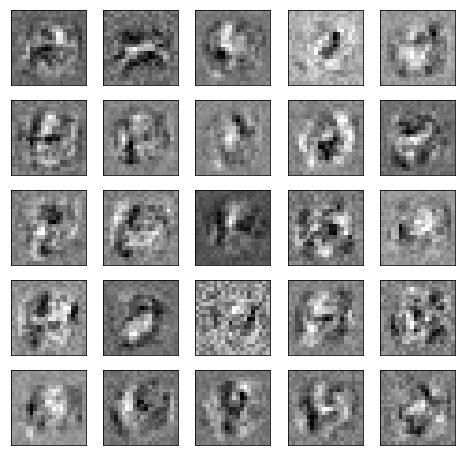
The code of visual hidden layer is as follows:

#Visual hidden layer
def plot_hidden(weight):
  fig,ax_array = plt.subplots(5, 5, sharex=True, sharey=True, figsize=(6,6))  #Divide the parent graph into 5 * 5 subgraphs, set the size of the graph, and set True to share the x and y axis attributes in all subgraphs
  for r in range(5):
    for c in range(5):
      ax_array[r, c].matshow(weight[r * 5 + c].reshape(20, 20), cmap='gray_r')  #Draw a digital image. cmap sets the drawing style to black characters on white background
      plt.xticks([])  #Remove scale to ensure beautiful appearance
      plt.yticks([])
  plt.show()

params = list(net.named_parameters()) #Obtain neural network parameters
plot_hidden(params[0][1].data)  #Get hidden layer parameters and visualize them

(conclusion personal diary: it's June unconsciously. I still can't go back to school. I can't see the people I want to see. But the happy thing is that this week, the tutor is finally determined, and it's the tutor you want at the beginning after making a choice. At the end of last semester, I sent an email, but there was no real progress. During the epidemic, I struggled to contact my teacher at the beginning of school. At last, I sorted out my resume for one day on an impulse day, and sent it to my teacher. At least, I brush the existence feeling and let the teacher know about myself. Unexpectedly, the teacher agreed to ha ha ha, which was a surprise. Maybe sometimes you really can't think too much about it. Only by taking action can you have the chance to push things forward (cover your face manually)