1. Process

1. Software download and installation
2. data acquisition
3. Custom dataset
4. Model building
5. model training
6. test
7. summary
8. follow-up

Download address of this project GitHub

1. Software download and installation

1.Download address: https://github.com/udacity/self-driving-car-sim
2. After entering the link, you can choose your own platform to download.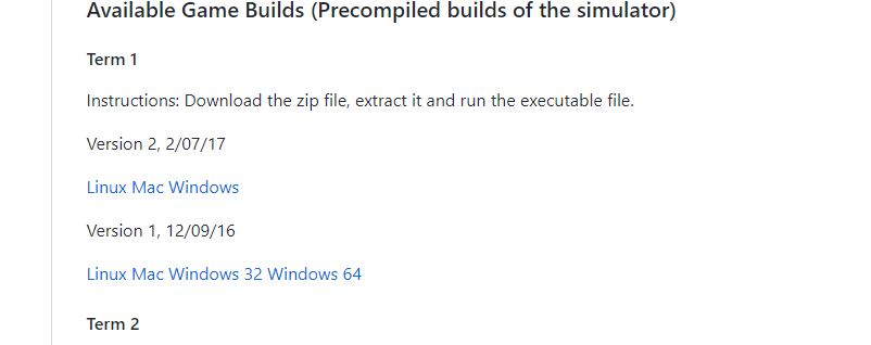
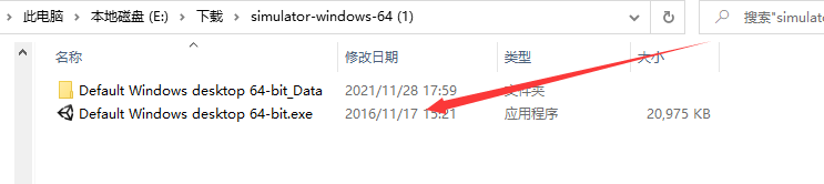
3. The downloaded package is a compressed package, which can be directly decompressed for use

2. Data acquisition

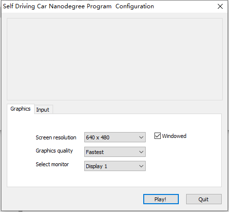
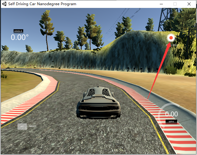
1. After the software is opened, there will be an interface as shown in the figure, that is, select resolution, image quality and display. If your computing resources are limited, it is recommended to select the parameters shown in the figure. Otherwise, a large delay will occur when the computing resources cannot be reached. It is not recommended here.
   

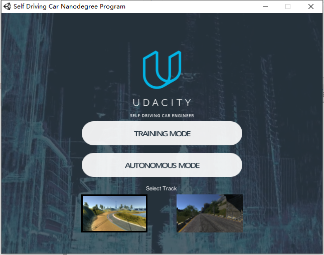
2. After entering, you will be allowed to select training mode and autonomous mode, namely training mode and automatic driving mode. In the data acquisition stage, you must select training mode, which is actually data acquisition.
   

3. After entering the training mode, click the button as shown in the figure to select the data storage path, and then click again to collect data
   

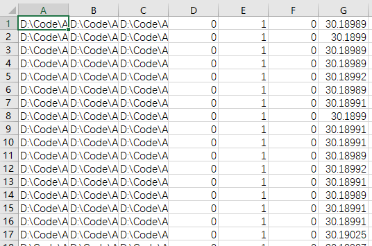
4. After the acquisition, these two files will be generated in the folder you select. IMG is the picture taken by the three cameras in front of the car, and driving.csv is the parameter of each picture
   

5. As shown in the figure, the csv files are the pictures taken by the middle camera, the left camera and the right camera, followed by the steering angle, throttle size, brake size and current speed.
   

3. Data enhancement

1. Why do you do this? If you do the steering data histogram once, you can see that the data you want to turn left is significantly larger than the data you want to turn right, and the data you don't turn is much larger than the steering data, and the image data collected manually is limited.
   
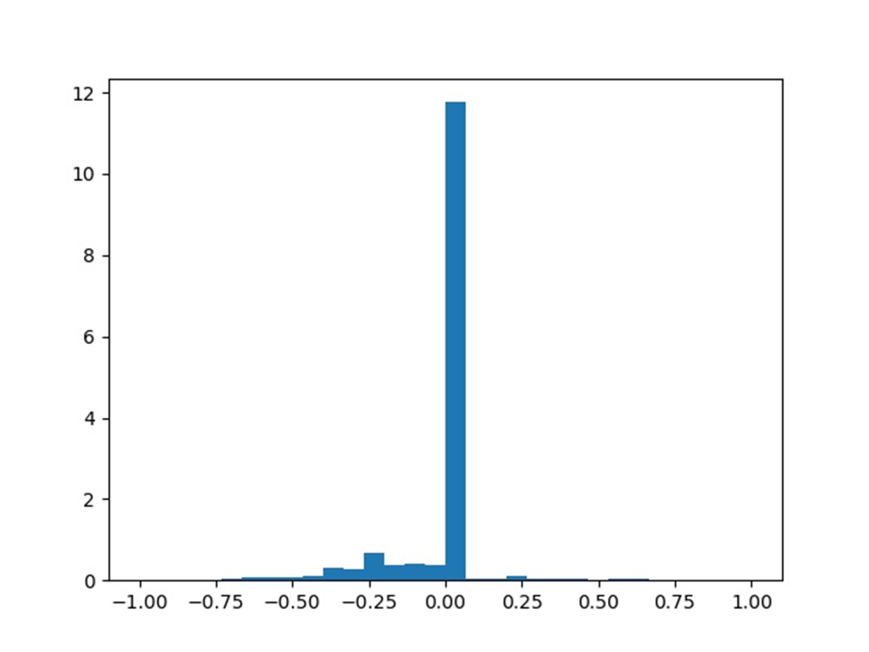
2. All you need to do is flip the horizontal mirror image of the image, remove the part and turn to the value of 0. And the value random transformation of HSV color space.

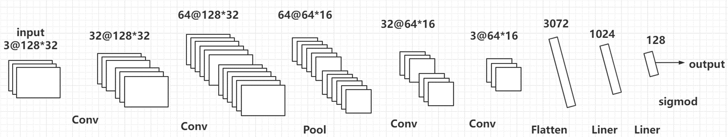
4. Model construction

1. The model is shown in the figure. It is a very simple model, but the parameters are sufficient for this project.
   

class CustomerNet(nn.Module):
    def __init__(self):
        super(CustomerNet,self).__init__()
        self.conv2d0=nn.Conv2d(in_channels=3,out_channels=32,kernel_size=5,stride=1,padding=2,bias=True)
        self.conv2d1=nn.Conv2d(in_channels=32,out_channels=32,kernel_size=5,stride=1,padding=2,bias=True)
        self.conv2d2=nn.Conv2d(in_channels=32,out_channels=64,kernel_size=5,stride=1,padding=2,bias=True)
        self.maxpool0=nn.MaxPool2d(kernel_size=2,stride=2,padding=0)
        self.conv2d3=nn.Conv2d(in_channels=64,out_channels=32,kernel_size=5,stride=1,padding=2,bias=True)
        self.conv2d4=nn.Conv2d(in_channels=32,out_channels=3,kernel_size=5,stride=1,padding=0,bias=True)
        self.flatten1=nn.Flatten()
        self.relu=nn.ReLU()
        self.liner1=nn.Linear(in_features=2160,out_features=320)
        self.liner2=nn.Linear(in_features=320,out_features=80)
        self.liner3=nn.Linear(in_features=80,out_features=20)
        self.liner4=nn.Linear(in_features=20,out_features=1)

        self.liner11=nn.Linear(in_features=4096,out_features=1024)
        self.liner22=nn.Linear(in_features=1024,out_features=128)
        self.liner33=nn.Linear(in_features=128,out_features=1)


    def forward(self,x):
        x=self.relu(self.conv2d0(x))
        x=self.maxpool0(x)
        x=self.relu(self.conv2d1(x))
        x=self.maxpool0(x)
        x=self.relu(self.conv2d2(x))
        x=self.maxpool0(x)
        x=self.relu(self.flatten1(x))
        # print(x.shape)
        x=F.relu(self.liner11(x))
        x=self.relu(self.liner22(x))
        x=self.liner33(x)
        return x

5. Model training

1. This step can follow the general process. Because the model is very small, training with cpu will be very fast. At the same time, the training will generate logs during the training in the logs directory

def main():
    model=CustomerNet()
    #Load loss function
    # loss=nn.CrossEntropyLoss()
    loss=nn.MSELoss()
    #Load optimizer
    optmizer=opt.SGD(model.parameters(),lr=0.003,momentum=0.8)
    # trans=transforms.Compose([transforms.ToTensor()])
    train_data,val_data,test_data=load_train_val(1)
    sumwriter=SummaryWriter(log_dir='../logs')
    #Training theory number
    epochs=80
    step=1
    for epoch in range(epochs):
        print(f'-------------The first{epoch+1}Round training-----------')
        runing_loss = 0
        ind=0
        train_data, val_data, test_data = load_train_val(0.8)
        random.shuffle(train_data)
        for data in tqdm(train_data):
            try:imgpath,lables=data
            except:continue
            lables=torch.from_numpy(np.array([float(lables)],dtype=np.float32))
            #Image preprocessing
            img=trans_data(imgpath)
            optmizer.zero_grad()
            netout=model(img)
            # print(lables)
            lossnow=loss(netout,lables)
            lossnow.backward()
            optmizer.step()
            runing_loss+=lossnow.item()
            ind += 1
            if ind%1000==0:
                print('<<<<--------The first%3d round,Picture:%10d Zhang---------->>>> loss:%3f' %(epoch+1,ind,runing_loss/1000))
                # sumwriter.add_image('img',img,dataformats='CWH')
                sumwriter.add_scalar(tag='Loss',scalar_value=runing_loss/1000,global_step=step)
                step+=1
                if runing_loss/1000==0:
                    save(model,epoch)
                    return
                runing_loss = 0
        save(model,epoch)

6. Test

That's enough. Let's see the effect directly.
Station B address:https://www.bilibili.com/video/BV1Kf4y1K7z2/

7. Summary

Let's talk about what I learned from this experiment. I tried it again and again myself.

1. Data enhancement is very necessary. Before training, we must observe the overall data for subsequent processing. Effective data processing can get twice the result with half the effort
2. Without ReLu activation function, over fitting will occur.
3. Too much learning rate will lead to losses and violent shocks
4. If the learning rate is too small, the gradient will disappear
5. It took me three and a half days to say a little episode. It took me more than two hours to write the code. Later, it was all parameter debugging, so I got the above summary. It was mainly in the part of image cutting. I originally cut down 60 pixels. I didn't think there was anything here after training several times. Finally, I couldn't find anything to change, so I changed it here, After changing 60 to 65, the training effect is surprisingly good. So data processing is really important.

8. Follow up

1. At present, the code of YOLOv1 is coming to an end, and the subsequent code will also be uploaded to GitHub. Please pay attention and make progress together.