[artificial intelligence project] Fashion Mnist recognition experiment
This paper mainly carries out the recognition experiment of fashion mnist through four methods, mainly including word bag model, hog feature, mlp multilayer perceptron and cnn convolution neural network. Then don't say much, get up!!!

Fashion Mnist
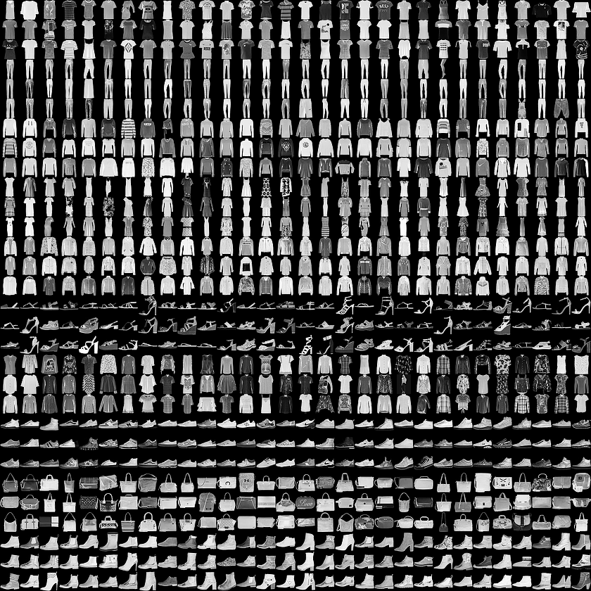
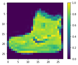
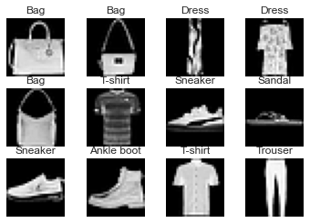
Fashion MNIST is an image data set containing 70000 gray images covering 10 categories (T-shirts, shoes, etc.). The following image shows the effect of a single dress at a lower resolution (28x28 pixels):
What will be done next?
1, Import Fashion Mnist
1. Import module
# Import library
import tensorflow as tf
from tensorflow import keras

import numpy as np
import matplotlib.pyplot as plt
D:\software\Anaconda\anaconda\envs\tensorflow\lib\site-packages\tensorflow\python\framework\dtypes.py:516: FutureWarning: Passing (type, 1) or '1type' as a synonym of type is deprecated; in a future version of numpy, it will be understood as (type, (1,)) / '(1,)type'.
  _np_qint8 = np.dtype([("qint8", np.int8, 1)])
D:\software\Anaconda\anaconda\envs\tensorflow\lib\site-packages\tensorflow\python\framework\dtypes.py:517: FutureWarning: Passing (type, 1) or '1type' as a synonym of type is deprecated; in a future version of numpy, it will be understood as (type, (1,)) / '(1,)type'.
  _np_quint8 = np.dtype([("quint8", np.uint8, 1)])
D:\software\Anaconda\anaconda\envs\tensorflow\lib\site-packages\tensorflow\python\framework\dtypes.py:518: FutureWarning: Passing (type, 1) or '1type' as a synonym of type is deprecated; in a future version of numpy, it will be understood as (type, (1,)) / '(1,)type'.
  _np_qint16 = np.dtype([("qint16", np.int16, 1)])
D:\software\Anaconda\anaconda\envs\tensorflow\lib\site-packages\tensorflow\python\framework\dtypes.py:519: FutureWarning: Passing (type, 1) or '1type' as a synonym of type is deprecated; in a future version of numpy, it will be understood as (type, (1,)) / '(1,)type'.
  _np_quint16 = np.dtype([("quint16", np.uint16, 1)])
D:\software\Anaconda\anaconda\envs\tensorflow\lib\site-packages\tensorflow\python\framework\dtypes.py:520: FutureWarning: Passing (type, 1) or '1type' as a synonym of type is deprecated; in a future version of numpy, it will be understood as (type, (1,)) / '(1,)type'.
  _np_qint32 = np.dtype([("qint32", np.int32, 1)])
D:\software\Anaconda\anaconda\envs\tensorflow\lib\site-packages\tensorflow\python\framework\dtypes.py:525: FutureWarning: Passing (type, 1) or '1type' as a synonym of type is deprecated; in a future version of numpy, it will be understood as (type, (1,)) / '(1,)type'.
  np_resource = np.dtype([("resource", np.ubyte, 1)])
D:\software\Anaconda\anaconda\envs\tensorflow\lib\site-packages\tensorboard\compat\tensorflow_stub\dtypes.py:541: FutureWarning: Passing (type, 1) or '1type' as a synonym of type is deprecated; in a future version of numpy, it will be understood as (type, (1,)) / '(1,)type'.
  _np_qint8 = np.dtype([("qint8", np.int8, 1)])
D:\software\Anaconda\anaconda\envs\tensorflow\lib\site-packages\tensorboard\compat\tensorflow_stub\dtypes.py:542: FutureWarning: Passing (type, 1) or '1type' as a synonym of type is deprecated; in a future version of numpy, it will be understood as (type, (1,)) / '(1,)type'.
  _np_quint8 = np.dtype([("quint8", np.uint8, 1)])
D:\software\Anaconda\anaconda\envs\tensorflow\lib\site-packages\tensorboard\compat\tensorflow_stub\dtypes.py:543: FutureWarning: Passing (type, 1) or '1type' as a synonym of type is deprecated; in a future version of numpy, it will be understood as (type, (1,)) / '(1,)type'.
  _np_qint16 = np.dtype([("qint16", np.int16, 1)])
D:\software\Anaconda\anaconda\envs\tensorflow\lib\site-packages\tensorboard\compat\tensorflow_stub\dtypes.py:544: FutureWarning: Passing (type, 1) or '1type' as a synonym of type is deprecated; in a future version of numpy, it will be understood as (type, (1,)) / '(1,)type'.
  _np_quint16 = np.dtype([("quint16", np.uint16, 1)])
D:\software\Anaconda\anaconda\envs\tensorflow\lib\site-packages\tensorboard\compat\tensorflow_stub\dtypes.py:545: FutureWarning: Passing (type, 1) or '1type' as a synonym of type is deprecated; in a future version of numpy, it will be understood as (type, (1,)) / '(1,)type'.
  _np_qint32 = np.dtype([("qint32", np.int32, 1)])
D:\software\Anaconda\anaconda\envs\tensorflow\lib\site-packages\tensorboard\compat\tensorflow_stub\dtypes.py:550: FutureWarning: Passing (type, 1) or '1type' as a synonym of type is deprecated; in a future version of numpy, it will be understood as (type, (1,)) / '(1,)type'.
  np_resource = np.dtype([("resource", np.ubyte, 1)])
The skeleton program for downloading and loading the fashion MNIST dataset has been integrated in tf.keras. You only need to import and load the data. 60000 pictures in the dataset are used to train the network, and 10000 pictures are used to evaluate the accuracy of the learned network classification images
Note: in machine learning, we generally divide the data set into training data set and test data set according to the ratio of 8:2. The training data set is used to train the model, and the test data set is used to test the accuracy of the trained model
2. Load dataset
# Load dataset
fashion_mnist = keras.datasets.fashion_mnist

(train_images, train_labels), (test_images, test_labels) = fashion_mnist.load_data()
After loading the dataset, four Numpy arrays will be returned
- train_images and train_ The labels array is the training set, that is, the data used for learning the model, with a total of 60000 pieces
- Test set test_images and test_ The labels array is used to test the model. There are 10000 in total
- train_images and test_ All images are 28x28 NumPy arrays, and the value of each point is between 0 and 255. Represents the current picture_ Images and test_labels is a 10 dimensional array of integers, and the value of each dimension is between 0 and 9. The labels representing the current image correspond to the category of the clothing represented by the image:
3. Explore data sets
#We first explore the format of the data set, and then train the model. Let's first look at the shape of the pictures in the dataset
print(train_images.shape)
(60000, 28, 28)
#Let's take another look at the shape of the label in the dataset
print(train_labels.shape)
(60000,)
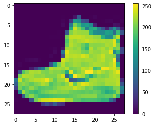
# visualization
## Create a new image
plt.figure()
## Display image (fill in image)
plt.imshow(train_images[0])
## Add a colorbar (color bar or gradient bar) to the subgraph
plt.colorbar()
## Set gridlines
plt.grid(False)
4. View labels
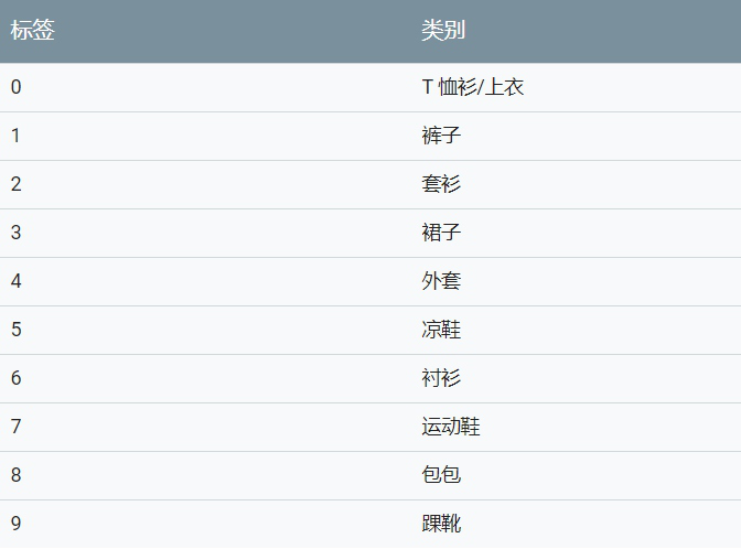
class_names = ['T-shirt/top', 'Trouser', 'Pullover', 'Dress', 'Coat',
               'Sandal', 'Shirt', 'Sneaker', 'Bag', 'Ankle boot']
print(train_labels[0])
print(class_names[train_labels[0]])
9
Ankle boot
5. Preprocessing normalization operation
We reduce these values in the picture to between 0 and 1, and then feed them to the neural network model. To do this, the data type of the image component is converted from an integer to a floating point number, and then divided by 255. This makes it easier to train. The following is the function of preprocessing images: it is important to preprocess the training set and the test set in the same way:
train_images = train_images / 255.0
test_images = test_images / 255.0
# Display the image after preprocessing
plt.figure()
plt.imshow(train_images[0])
plt.colorbar()
plt.grid(False)
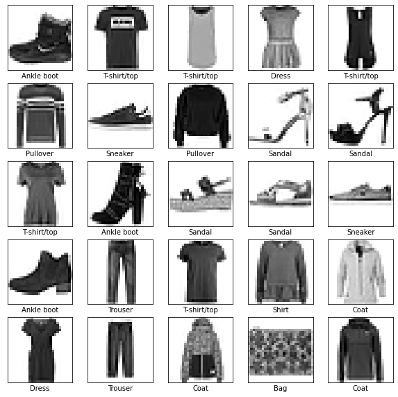
#The first 25 images in the training set are displayed, and the category name is displayed under each image. Verify that the data format is correct, and then we can start building and training the network.
plt.figure(figsize=(10,10))
for i in range(25):
    ## Generate 5 * 5 subgraphs under the current graph
    plt.subplot(5,5,i+1)
    plt.xticks([])
    plt.yticks([])
    plt.grid(False)
    plt.imshow(train_images[i], cmap=plt.cm.binary)
    #Displays the category of the current picture
    plt.xlabel(class_names[train_labels[i]])
2, Based on word bag model
- (1) The feature points of each image are still extracted, such as SIFT feature points
- (2) For all SIFT feature points of all pictures, kmeans clustering is carried out as a whole, and the words are divided into multiple different classes. The number of classes is defined as wordCount.
- (3) For each picture, calculate the number of SIFT features of different classes, corresponding to one dimension of the feature vector to be obtained. Then we can generate a vector of wordCount dimension for each picture.
Steps to obtain the BoW vector of an image:
- Visual dictionary for constructing image library
- Extract the local features of all images in the image library, such as SIFT
- Cluster the extracted image features, such as k-means, and get that the clustering center is the visual Vocabulary dictionary of the image database
- Calculate the BoW vector of an image
- Extract local features of image
- Count the frequency of each visual word in Vocabulay in the image.
import os
import cv2
import pickle
import numpy as np
import matplotlib.pyplot as plt
from imutils import paths
from sklearn.cluster import KMeans
from scipy.cluster.vq import vq
from sklearn.model_selection import train_test_split

from sklearn.svm import LinearSVC
print(train_images.shape)
print(train_labels.shape)
print(test_images.shape)
print(test_labels.shape)
(60000, 28, 28)
(60000,)
(10000, 28, 28)
(10000,)
sifts_img = [] # The file names and sift features of all images are stored

limit = 10000 #Maximum number of training

count = 0 # Number of word bag features
num = 0 # Effective number
label = []
for i in range(limit):
    img = train_images[i].reshape(28,28)
    img = np.uint8(np.double(img) * 255)
    sift = cv2.xfeatures2d.SIFT_create()
    kp,des = sift.detectAndCompute(img,None)
    if des is None:
        continue
    sifts_img.append(des)
    label.append(train_labels[i])
    count = count + des.shape[0]
    num = num + 1

label = np.array(label)

data = sifts_img[0]
for des in sifts_img[1:]:
    data = np.vstack((data, des))

print("train file:",num)
count = int(count / 40)
count = max(4,count)
train file: 9236
# Clustering sift features
k_means = KMeans(n_clusters=int(count), n_init=4)
k_means.fit(data)


# Construct the word bag representation of all samples
image_features = np.zeros([int(num),int(count)],'float32')
for i in range(int(num)):
    ws, d = vq(sifts_img[i],k_means.cluster_centers_)# Calculate the visual vocabulary of each sift feature
    for w in ws:
        image_features[i][w] += 1  # Add 1 to the corresponding visual vocabulary position element


x_tra, x_val, y_tra, y_val = train_test_split(image_features,label,test_size=0.2)
# Construct linear SVM objects and train them
clf = LinearSVC(C=1, loss="hinge").fit(x_tra, y_tra)
# Prediction accuracy of training data
print (clf.score(x_val, y_val))


# save the training model as pickle
with open('bow_kmeans.pickle','wb') as fw:
    pickle.dump(k_means,fw)
with open('bow_clf.pickle','wb') as fw:
    pickle.dump(clf,fw)
with open('bow_count.pickle','wb') as fw:
    pickle.dump(count,fw)
print('Trainning successfully and save the model')
0.6293290043290043
Trainning successfully and save the model


D:\software\Anaconda\anaconda\envs\tensorflow\lib\site-packages\sklearn\svm\_base.py:947: ConvergenceWarning: Liblinear failed to converge, increase the number of iterations.
  "the number of iterations.", ConvergenceWarning)
with open('bow_kmeans.pickle','rb') as fr:
k_means = pickle.load(fr)
with open('bow_clf.pickle','rb') as fr:
clf = pickle.load(fr)
with open('bow_count.pickle','rb') as fr:
count = pickle.load(fr)
target_file = ['T-shirt','Trouser','Pullover',
'Dress','Coat','Sandal','Shirt',
'Sneaker','Bag','Ankle boot']
plt.figure()
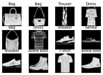
cnt = 30
i = 1
while(i<=12):
img = test_images[cnt].reshape(28,28)
cnt = cnt + 1
img = np.uint8(np.double(img) * 255)
sift = cv2.xfeatures2d.SIFT_create()
kp,des = sift.detectAndCompute(img,None)
if des is None:
continue
words, distance = vq(des, k_means.cluster_centers_)
image_features_search = np.zeros((int(count)), "float32")
for w in words:
image_features_search[w] += 1
t = clf.predict(image_features_search.reshape(1,-1))
plt.subplot(3,4,i)
i += 1
plt.imshow(img,'gray')
plt.title(target_file[t[0]])
plt.axis('off')
plt.show()
with open('bow_kmeans.pickle','rb') as fr:
    k_means = pickle.load(fr)
with open('bow_clf.pickle','rb') as fr:
    clf = pickle.load(fr)
with open('bow_count.pickle','rb') as fr:
    count = pickle.load(fr)


i = 0
len = test_images.shape[0]
predict_arr = []

while(i<len):
    img = test_images[i].reshape(28,28)
    img = np.uint8(np.double(img) * 255)
    sift = cv2.xfeatures2d.SIFT_create()
    print(i)
    kp,des = sift.detectAndCompute(img,None)
    if des is None:
        i += 1
        predict_arr.append(0)
        continue
    words, distance = vq(des, k_means.cluster_centers_)
    image_features_search = np.zeros((int(count)), "float32")
    for w in words:
        image_features_search[w] += 1
    t = clf.predict(image_features_search.reshape(1,-1))
    i += 1
    predict_arr.append(t[0])
0
1
2
3
4
5
6
7
8
9
10
11
12
13
14
15
16
17
18
19
20
21
22
23
24
25
26
27
28
29
30
31
32
33
34
35


9995
9996
9997
9998
9999
from sklearn.metrics import accuracy_score,f1_score,confusion_matrix,classification_report

score=accuracy_score(test_labels,predict_arr)
print(score)
0.5651
print(classification_report(test_labels,predict_arr))
              precision    recall  f1-score   support

           0       0.36      0.60      0.45      1000
           1       0.72      0.47      0.57      1000
           2       0.43      0.47      0.45      1000
           3       0.49      0.46      0.47      1000
           4       0.45      0.44      0.44      1000
           5       0.79      0.74      0.76      1000
           6       0.36      0.24      0.29      1000
           7       0.74      0.74      0.74      1000
           8       0.67      0.66      0.66      1000
           9       0.79      0.84      0.81      1000

    accuracy                           0.57     10000
   macro avg       0.58      0.57      0.56     10000
weighted avg       0.58      0.57      0.56     10000
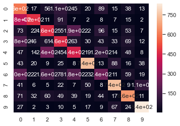
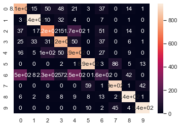
import seaborn as sns
from sklearn.metrics import confusion_matrix
import matplotlib.pyplot as plt
%matplotlib inline
sns.set()

# Confusion matrix


matrix = confusion_matrix(test_labels,predict_arr)
print(matrix)
sns.heatmap(matrix,annot=True)
[[598  17  56 109  45  20  89  15  38  13]
 [384 473  11  91   7   2   8   7  15   2]
 [ 73  22 465  55 192  22  96  15  53   7]
 [184  46  61 459  63  30  43  33  69  12]
 [ 47  14 245  45 441  19 119  14  48   8]
 [ 43  20   9  25   8 740  13  88  16  38]
 [205  22 161  78 184  23 238  11  59  19]
 [ 41   6   5  22   7  50   8 743   9 109]
 [ 71  32  60  49  39  19  44  17 658  11]
 [ 27   2   3  10   5  17   9  67  24 836]]


<matplotlib.axes._subplots.AxesSubplot at 0x1f384714548>
3, Based on HOG feature
Histogram of Oriented Gridients, abbreviated as HOG, is a feature commonly used in the field of computer vision and pattern recognition to describe the local texture of an image. The feature name is also very straightforward, that is, first calculate the gradient values in different directions in an area of the picture, and then accumulate them to obtain a histogram. This histogram can represent this area, that is, as a feature, it can be input into the classifier. Then, let's introduce the specific principle and calculation method of HOG, as well as some extensions.
Because HOG is a local feature, you can't get good results if you directly extract features from a large image. The principle is simple. From the perspective of information theory, for example, a 640 * 480 image has about 300000 pixels, that is, the original data has 300000 dimensional features. If HOG is directly done, even if it is divided into 360 bin s according to 360 degrees, it does not have the ability to represent such a large image. From the perspective of Feature Engineering, generally speaking, only when the image area is relatively small, the histogram based on statistical principle can express the area. If the image area is relatively large, the HOG features of two completely different images may also be very similar. However, if the area is small, this possibility is very small. Finally, the image is divided into many blocks, and then the HOG feature is calculated for each block, which also includes geometric (position) characteristics. For example, for a frontal face, the HOG feature extracted from the image block in the upper left part is generally consistent with the HOG feature of the eye.
import warnings
warnings.filterwarnings("ignore")

import os
import cv2
import pickle
import numpy as np
import matplotlib.pyplot as plt
from imutils import paths
from skimage.feature import hog
from scipy.cluster.vq import vq
from sklearn.svm import LinearSVC
from sklearn.model_selection import train_test_split
limit = train_images.shape[0]

data = [] # HoG characteristics
label = []
for i in range(limit):
    img = train_images[i].reshape(28,28)
    img = np.uint8(np.double(img) * 255)
    fd = hog(img)
    data.append(fd)
    label.append(train_labels[i])

data = np.array(data)
label = np.array(label)

x_tra, x_val, y_tra, y_val = train_test_split(data,label,test_size=0.2)

print('train file:',y_tra.size)
print('val file:',y_val.size)

# Construct linear SVM objects and train them
clf = LinearSVC(C=1, loss="hinge").fit(x_tra, y_tra)
# Prediction accuracy of training data
print ('accuracy:',clf.score(x_val, y_val))


# save the training model as pickle
with open('hog.pickle','wb') as fw:
    pickle.dump(clf,fw)
print('Trainning successfully and save the model')
train file: 48000
val file: 12000
accuracy: 0.799
Trainning successfully and save the model
with open('hog.pickle','rb') as fr:
    clf = pickle.load(fr)

target_file = ['T-shirt','Trouser','Pullover',
               'Dress','Coat','Sandal','Shirt',
               'Sneaker','Bag','Ankle boot']

plt.figure()
cnt = 30
i = 1
while(i<=12):
    img = test_images[cnt].reshape(28,28)
    cnt = cnt + 1
    img = np.uint8(np.double(img) * 255)
    fd = hog(img)
    t = clf.predict([fd])
    plt.subplot(3,4,i)
    i += 1
    plt.imshow(img,'gray')
    plt.title(target_file[t[0]])
    plt.axis('off')
plt.show()

with open('hog.pickle','rb') as fr:
    clf = pickle.load(fr)


i = 0
len = test_images.shape[0]
predict_arr = []

while(i<len):
    img = test_images[i].reshape(28,28)
    img = np.uint8(np.double(img) * 255)
    fd = hog(img)
    t = clf.predict([fd])
    i += 1
    predict_arr.append(t[0])
from sklearn.metrics import accuracy_score,f1_score,confusion_matrix,classification_report

score=accuracy_score(test_labels,predict_arr)
print(score)
0.7904
print(classification_report(test_labels,predict_arr))
              precision    recall  f1-score   support

           0       0.70      0.81      0.75      1000
           1       0.94      0.94      0.94      1000
           2       0.62      0.71      0.67      1000
           3       0.79      0.82      0.81      1000
           4       0.61      0.79      0.69      1000
           5       0.92      0.89      0.90      1000
           6       0.47      0.16      0.24      1000
           7       0.87      0.90      0.88      1000
           8       0.91      0.94      0.92      1000
           9       0.94      0.94      0.94      1000

    accuracy                           0.79     10000
   macro avg       0.78      0.79      0.77     10000
weighted avg       0.78      0.79      0.77     10000
import seaborn as sns
from sklearn.metrics import confusion_matrix
import matplotlib.pyplot as plt
%matplotlib inline
sns.set()

# Confusion matrix


matrix = confusion_matrix(test_labels,predict_arr)
print(matrix)
sns.heatmap(matrix,annot=True)
[[811  15  50  48  21   3  37   0  14   1]
 [  3 943  10  32   4   0   7   0   1   0]
 [ 37   1 715  15 166   1  51   0  14   0]
 [ 25  33  31 817  50   0  37   0   6   1]
 [ 16   5 103  50 790   0  27   0   9   0]
 [  0   0   0   2   1 890   3  86   5  13]
 [253   8 228  57 253   0 159   0  42   0]
 [  0   0   0   0   0  59   1 897   1  42]
 [  6   2   8   8   9   8  13   2 943   1]
 [  0   0   0   0   0  10   2  45   4 939]]


<matplotlib.axes._subplots.AxesSubplot at 0x1f382c92408>
4, MLP multilayer perceptron
MLP (Multilayer Perceptron) is also called Artificial Neural Network (ANN). In addition to the input and output layer, it can have multiple hidden layers. The simplest MLP contains only one hidden layer, that is, a three-layer structure
import numpy as np
from keras.models import Sequential
from keras.layers import Dense, Dropout, Flatten, Activation
from keras.layers import Conv2D, MaxPooling2D
from keras.utils.vis_utils import plot_model
from keras.utils import np_utils
X_train = train_images.reshape((-1,784))
X_test = test_images.reshape(-1,784)
Y_train = np_utils.to_categorical(train_labels,num_classes=10)
Y_test = np_utils.to_categorical(test_labels,num_classes=10)
# Build MLP
model = Sequential()

model.add(Dense(units=256,
                input_dim=784,
                kernel_initializer='normal',
                activation='relu'))

model.add(Dense(units=10,
                kernel_initializer='normal',
                activation='softmax'))

model.summary()
_________________________________________________________________
Layer (type)                 Output Shape              Param #
=================================================================
dense_3 (Dense)              (None, 256)               200960
_________________________________________________________________
dense_4 (Dense)              (None, 10)                2570
=================================================================
Total params: 203,530
Trainable params: 203,530
Non-trainable params: 0
_________________________________________________________________
model.compile(loss='categorical_crossentropy', optimizer='adam', metrics=['accuracy'])
model.fit(X_train, Y_train, batch_size=500, epochs=10, verbose=1, validation_data=(X_test, Y_test))
model.save('mlp_fashion_mnist.h5')
WARNING:tensorflow:From D:\software\Anaconda\anaconda\envs\tensorflow\lib\site-packages\tensorflow\python\ops\math_grad.py:1250: add_dispatch_support.<locals>.wrapper (from tensorflow.python.ops.array_ops) is deprecated and will be removed in a future version.
Instructions for updating:
Use tf.where in 2.0, which has the same broadcast rule as np.where
WARNING:tensorflow:From D:\software\Anaconda\anaconda\envs\tensorflow\lib\site-packages\keras\backend\tensorflow_backend.py:977: The name tf.assign_add is deprecated. Please use tf.compat.v1.assign_add instead.

Train on 60000 samples, validate on 10000 samples
Epoch 1/10
60000/60000 [==============================] - 28s 459us/step - loss: 0.6751 - acc: 0.7771 - val_loss: 0.4986 - val_acc: 0.8310
Epoch 2/10
60000/60000 [==============================] - 1s 19us/step - loss: 0.4437 - acc: 0.8480 - val_loss: 0.4469 - val_acc: 0.8400
Epoch 3/10
60000/60000 [==============================] - 2s 31us/step - loss: 0.3997 - acc: 0.8609 - val_loss: 0.4300 - val_acc: 0.8481
Epoch 4/10
60000/60000 [==============================] - 1s 18us/step - loss: 0.3749 - acc: 0.8682 - val_loss: 0.4151 - val_acc: 0.8546
Epoch 5/10
60000/60000 [==============================] - 1s 18us/step - loss: 0.3512 - acc: 0.8767 - val_loss: 0.3819 - val_acc: 0.8646
Epoch 6/10
60000/60000 [==============================] - 1s 19us/step - loss: 0.3345 - acc: 0.8819 - val_loss: 0.3882 - val_acc: 0.8625
Epoch 7/10
60000/60000 [==============================] - 1s 19us/step - loss: 0.3224 - acc: 0.8855 - val_loss: 0.3654 - val_acc: 0.8725
Epoch 8/10
60000/60000 [==============================] - 1s 19us/step - loss: 0.3086 - acc: 0.8889 - val_loss: 0.3558 - val_acc: 0.8723
Epoch 9/10
60000/60000 [==============================] - 1s 18us/step - loss: 0.2980 - acc: 0.8926 - val_loss: 0.3548 - val_acc: 0.8744
Epoch 10/10
60000/60000 [==============================] - 1s 19us/step - loss: 0.2879 - acc: 0.8963 - val_loss: 0.3560 - val_acc: 0.8719
from keras.models import load_model
model = load_model('mlp_fashion_mnist.h5')
plt.figure()
cnt = 30
i = 1
while(i<=12):
    img = [X_test[cnt]]
    cnt = cnt + 1
    img = np.uint8(np.double(img) * 255)
    t = model.predict(img)
    result = np.argmax(t, axis=1)
    plt.subplot(3,4,i)
    i += 1
    plt.imshow(img[0].reshape(28,28),'gray')
    plt.title(target_file[result[0]])
    plt.axis('off')
plt.show()
loss, accuracy = model.evaluate(X_test, Y_test, verbose=0)
print('loss:', loss)
print('accuracy:', accuracy)
loss: 0.35601275362968443
accuracy: 0.8719
predict = model.predict_classes(X_test)

from sklearn.metrics import accuracy_score,f1_score,confusion_matrix,classification_report

score=accuracy_score(test_labels,predict)
print(score)
0.8719
print(classification_report(test_labels,predict))
              precision    recall  f1-score   support

           0       0.81      0.86      0.83      1000
           1       0.97      0.97      0.97      1000
           2       0.79      0.74      0.76      1000
           3       0.85      0.90      0.87      1000
           4       0.72      0.87      0.79      1000
           5       0.97      0.94      0.96      1000
           6       0.78      0.55      0.65      1000
           7       0.93      0.95      0.94      1000
           8       0.96      0.97      0.96      1000
           9       0.95      0.96      0.96      1000

    accuracy                           0.87     10000
   macro avg       0.87      0.87      0.87     10000
weighted avg       0.87      0.87      0.87     10000
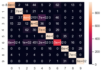
import seaborn as sns
from sklearn.metrics import confusion_matrix
import matplotlib.pyplot as plt
%matplotlib inline
sns.set()

# Confusion matrix


matrix = confusion_matrix(test_labels,predict)
print(matrix)
sns.heatmap(matrix,annot=True)
[[858   2  14  44   5   2  62   0  13   0]
 [  2 971   0  21   4   0   1   0   1   0]
 [ 22   3 739  15 173   0  46   0   2   0]
 [ 15  22  12 895  36   0  16   0   4   0]
 [  0   1  62  30 874   0  29   0   4   0]
 [  0   0   0   1   0 945   0  35   2  17]
 [161   4 100  45 123   0 551   0  16   0]
 [  0   0   0   0   0  16   0 955   0  29]
 [  4   1   7   4   6   3   0   5 970   0]
 [  0   0   0   0   0   7   1  31   0 961]]


<matplotlib.axes._subplots.AxesSubplot at 0x1f383b67a48>
5, CNN convolutional neural network
import numpy as np
from keras.models import Sequential
from keras.layers import Dense, Dropout, Flatten, Activation
from keras.layers import Conv2D, MaxPooling2D
from keras.utils.vis_utils import plot_model
from keras.utils import np_utils
X_train = train_images.reshape((-1,28,28,1))
X_test = test_images.reshape(-1,28,28,1)
Y_train = np_utils.to_categorical(train_labels,num_classes=10)
Y_test = np_utils.to_categorical(test_labels,num_classes=10)
# Build LeNet-5
model = Sequential()
model.add(Conv2D(filters=6, kernel_size=(5, 5), padding='valid', input_shape=(28, 28, 1), activation='relu')) # C1
model.add(MaxPooling2D(pool_size=(2, 2))) # S2
model.add(Conv2D(filters=16, kernel_size=(5, 5), padding='valid', activation='relu')) # C3
model.add(MaxPooling2D(pool_size=(2, 2))) # S4
model.add(Flatten())
model.add(Dense(120, activation='tanh')) # C5
model.add(Dense(84, activation='tanh')) # F6
model.add(Dense(10, activation='softmax')) # output
model.summary()
_________________________________________________________________
Layer (type)                 Output Shape              Param #
=================================================================
conv2d_3 (Conv2D)            (None, 24, 24, 6)         156
_________________________________________________________________
max_pooling2d_3 (MaxPooling2 (None, 12, 12, 6)         0
_________________________________________________________________
conv2d_4 (Conv2D)            (None, 8, 8, 16)          2416
_________________________________________________________________
max_pooling2d_4 (MaxPooling2 (None, 4, 4, 16)          0
_________________________________________________________________
flatten_2 (Flatten)          (None, 256)               0
_________________________________________________________________
dense_8 (Dense)              (None, 120)               30840
_________________________________________________________________
dense_9 (Dense)              (None, 84)                10164
_________________________________________________________________
dense_10 (Dense)             (None, 10)                850
=================================================================
Total params: 44,426
Trainable params: 44,426
Non-trainable params: 0
_________________________________________________________________
model.compile(loss='categorical_crossentropy', optimizer='adam', metrics=['accuracy'])
model.fit(X_train, Y_train, batch_size=500, epochs=10, verbose=1, validation_data=(X_test, Y_test))
model.save('cnn_fashion_mnist.h5')
Train on 60000 samples, validate on 10000 samples
Epoch 1/10
60000/60000 [==============================] - 3s 44us/step - loss: 0.3044 - acc: 0.8892 - val_loss: 0.3304 - val_acc: 0.8774
Epoch 2/10
60000/60000 [==============================] - 2s 34us/step - loss: 0.2902 - acc: 0.8948 - val_loss: 0.3259 - val_acc: 0.8809
Epoch 3/10
60000/60000 [==============================] - 2s 35us/step - loss: 0.2826 - acc: 0.8967 - val_loss: 0.3145 - val_acc: 0.8865
Epoch 4/10
60000/60000 [==============================] - 2s 33us/step - loss: 0.2724 - acc: 0.9002 - val_loss: 0.3158 - val_acc: 0.8862
Epoch 5/10
60000/60000 [==============================] - 2s 33us/step - loss: 0.2683 - acc: 0.9025 - val_loss: 0.3174 - val_acc: 0.8843
Epoch 6/10
60000/60000 [==============================] - 2s 34us/step - loss: 0.2610 - acc: 0.9047 - val_loss: 0.3040 - val_acc: 0.8900
Epoch 7/10
60000/60000 [==============================] - 2s 34us/step - loss: 0.2519 - acc: 0.9082 - val_loss: 0.3015 - val_acc: 0.8904
Epoch 8/10
60000/60000 [==============================] - 2s 33us/step - loss: 0.2481 - acc: 0.9086 - val_loss: 0.3097 - val_acc: 0.8877
Epoch 9/10
60000/60000 [==============================] - 2s 34us/step - loss: 0.2432 - acc: 0.9107 - val_loss: 0.2940 - val_acc: 0.8936
Epoch 10/10
60000/60000 [==============================] - 2s 34us/step - loss: 0.2355 - acc: 0.9134 - val_loss: 0.2934 - val_acc: 0.8924
loss, accuracy = model.evaluate(X_test, Y_test, verbose=0)
print('loss:', loss)
print('accuracy:', accuracy)
loss: 0.29342212826013564
accuracy: 0.8924
predict = model.predict_classes(X_test)

from sklearn.metrics import accuracy_score,f1_score,confusion_matrix,classification_report

score=accuracy_score(test_labels,predict)
print(score)
0.8924
print(classification_report(test_labels,predict))
              precision    recall  f1-score   support

           0       0.80      0.88      0.84      1000
           1       0.99      0.97      0.98      1000
           2       0.81      0.87      0.84      1000
           3       0.88      0.91      0.90      1000
           4       0.83      0.82      0.83      1000
           5       0.97      0.97      0.97      1000
           6       0.75      0.62      0.68      1000
           7       0.92      0.97      0.95      1000
           8       0.97      0.98      0.97      1000
           9       0.98      0.94      0.96      1000

    accuracy                           0.89     10000
   macro avg       0.89      0.89      0.89     10000
weighted avg       0.89      0.89      0.89     10000
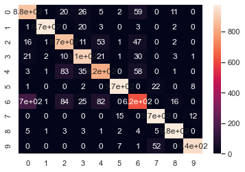
import seaborn as sns
from sklearn.metrics import confusion_matrix
import matplotlib.pyplot as plt
%matplotlib inline
sns.set()

# Confusion matrix


matrix = confusion_matrix(test_labels,predict)
print(matrix)
sns.heatmap(matrix,annot=True)
[[876   1  20  26   5   2  59   0  11   0]
 [  1 971   0  20   3   0   3   0   2   0]
 [ 16   1 869  11  53   1  47   0   2   0]
 [ 21   2  10 911  21   1  30   0   3   1]
 [  3   1  83  35 819   0  58   0   1   0]
 [  1   0   0   2   0 967   0  22   0   8]
 [170   1  84  25  82   0 622   0  16   0]
 [  0   0   0   0   0  15   0 973   0  12]
 [  5   1   3   3   1   2   4   5 976   0]
 [  0   0   0   0   0   7   1  52   0 940]]


<matplotlib.axes._subplots.AxesSubplot at 0x1f4444938c8>
Summary
So this experiment is over, praise comments collection one-stop, porcelain!!!!