Over fitting, under fitting and model generalization
This article contains a lot of content. I will introduce the over fitting, under fitting, model generalization and two models of Ridge regression and LASSO regression to optimize the over fitting
polynomial regression
We have mentioned simple linear regression and multiple linear regression before, which assume that there is a linear relationship between features and sample target value, but there are few scenes with simple linear relationship in practical application;
If the relationship between the feature and the target value is non-linear and the regression line is a curve, that is, there is a power function relationship between the target value and one or more features, how to predict the target value? This leads to polynomial regression;
The way to realize polynomial regression is very simple. Since we assume that there is a high power relationship between the target value and the feature, then we can calculate the power function value of all the features as a new feature to add to the feature, that is, we can upgrade the latitude of the data;
Example: y=ax2+bx+c
For example:
y = ax^2 + bx + c
Example: y=ax2+bx+c
Assuming the quadratic function model above, the feature latitude is 1, i.e. X; we can take x2x^2x2 as a new feature X1 = X2X_ 1 = x ^ 2x 1 = X2, which means that the feature latitude changes to 2,
y=ax1+bx2+c
y = ax_1 + bx_2 + c
y=ax1+bx2+c
Comfortable ~
Then, the multiple linear regression model is used to train and get the θ \ theta θ coefficients of each feature, thus realizing the polynomial regression
Here we generate a training data set
import matplotlib.pyplot as plt
import numpy as np

X = np.arange(-10,10,.1).reshape((-1,1))
# Relationship between target value and X feature y = 0.5x^3 - x^2 + x + 5 + noise
y = .5 * X[:,0]**3 - X[:,0]**2 + X[:,0] + 5 + np.random.normal(-50,50,200)
plt.scatter(X,y)
It's like the rainbow in the wolf disco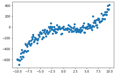
Next, we use the Pipeline provided by sklearn to assemble the data feature stack, data normalization and linear regression together to form a function that can train the polynomial regression model
- PolynomialFeatures are used to raise the latitude of a feature. The constructor passes in degree to add the most power of the feature to the feature
- Normalization of StandardScaler data for unifying feature dimensions
- Linear regression
# Divide the data sample into training data set and test data set
from sklearn.model_selection import train_test_split
X_train, X_test, y_train, y_test = train_test_split(X,y)
from sklearn.linear_model import LinearRegression
from sklearn.preprocessing import PolynomialFeatures
from sklearn.pipeline import Pipeline
from sklearn.preprocessing import StandardScaler

def polynomialFeatures(degree):
    return Pipeline([
        ("poly", PolynomialFeatures(degree=degree)),
        ("scaler", StandardScaler()),
        ("linear_reg", LinearRegression())
    ])
Over fitting, under fitting, generalization ability
We have manually generated training data sets, and we know that y and x have the highest cubic relationship
Next, I will try to train with the power of 1, the power of square, the power of three and the power of thirty
Furthermore, the phenomenon of over fitting and under fitting is expounded
# 1 power
poly1 = polynomialFeatures(degree=1)
poly1.fit(X_train, y_train)
y_pre1 = poly1.predict(X_train)
plt.scatter(X,y)
plt.plot(np.sort(X_train[:,0]), y_pre1[np.argsort(X_train[:,0])],color = "red")
plt.title("R_Squared: {}".format(poly1.score(X_test, y_test)), color="red")
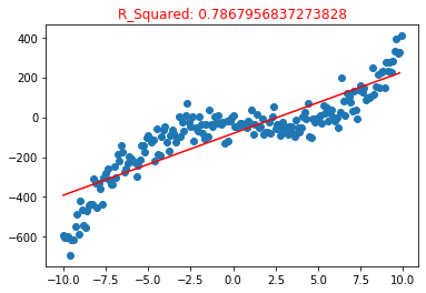
Since the highest power of the feature is used, it is equivalent to simple linear regression, so the regression line is a straight line
Use R_ The squared model is evaluated accurately, with an accuracy of 0.786, which is exactly the appearance of artificial mental retardation
This is the result of under fitting. In our training data set, the relationship between the feature and the target value is the highest third power, but the model we train is the first power. In other words, this model can not completely express the relationship between the feature and the target value, so the accuracy of the model is only 0.7
Here is the square polynomial regression model
poly2 = polynomialFeatures(degree = 2)
poly2.fit(X_train, y_train)
y_pre2 = poly2.predict(X_train)

plt.title("R_Squared: {}".format(poly2.score(X_test, y_test)),color = "red")
plt.scatter(X,y)
plt.plot(np.sort(X_train[:,0]),y_pre2[np.argsort(X_train[:,0])],color = "red")
Using the training data set with the square value of the feature to train the model, it looks like a little curve
But! However !
R_2. The accuracy of the model is 0.71, which is lower than the first power. From the perspective of image, it is also a product of under fitting
The following is the polynomial regression model trained by the training data set of the highest third power, which is consistent with the rules we generate
poly3 = polynomialFeatures(degree = 3)
poly3.fit(X_train, y_train)
y_pre3 = poly3.predict(X_train)

plt.title("R_Squared: {}".format(poly3.score(X_test, y_test)), color="red")
plt.scatter(X,y)
plt.plot(np.sort(X_train[:,0]), y_pre3[np.argsort(X_train[:,0])],color = "red")
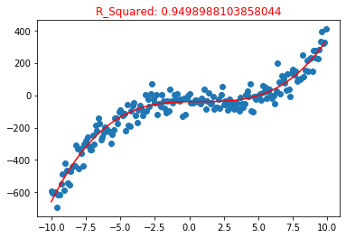
**excellent! **
The trained model at least perfectly matches the sample visually, R_2. The accuracy evaluation of the model also reached 0.94
Model error = deviation + variance + unavoidable error
Because of the noise in the process of training data set generation, the error is objective
Next, let's look at the case of over fitting. This time, we use the value of the highest 30 power of the feature to add the training data set as a new feature
poly5 = polynomialFeatures(degree =30)
poly5.fit(X_train, y_train)
y_pre5 = poly5.predict(X_train)

plt.title("R_Squared: {}".format(poly5.score(X_test, y_test)), color="red")
plt.scatter(X,y)
plt.plot(np.sort(X_train[:,0]), y_pre5[np.argsort(X_train[:,0])],color = "red")
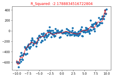
This regression curve is very fancy, winding, as if it fits very well, but it uses the test data set to evaluate the model accuracy R_2 = -2.17, when R_2 when the accuracy of the model is negative, it can be understood that the model is completely wrong, or even better to use the average value as the model for prediction;
Generalization ability
We can see that the curve fit is good. Why R_ The reason why the index is so low lies in over fitting: it fits the training sample well, but when it is applied to the production environment, the performance of the new sample prediction results is very poor. The model learns some irrelevant features, which is the over fitting situation. At the same time, it also shows that the generalization ability of the model is low, so it is difficult to generalize the model to the new sample
learning curve
Let's draw the learning curve of the above models; as the number of training samples increases, the trend of the model's prediction error for training samples and test samples will further explain the over fitting, under fitting, and generalization ability
In the following figures, the X-axis is the number of training samples, and the Y-axis is MSE (mean square error) to measure the error between the predicted value and the actual value. The larger the error is, the lower the accuracy of the model can be understood;
There are two lines in each picture, which can not only show the prediction error of the model to the training data set and the prediction error after generalization to the sample that does not exist in the training data set
from sklearn.metrics import mean_squared_error
# Draw model learning curve
def drawLearnLinear(func, X, y):
    X_train, X_test, y_train, y_test = train_test_split(X,y,test_size=0.3)
    train_mse = np.empty(len(X_train))
    test_mse = np.empty(len(X_train))
    for i in range(len(X_train)):
        func.fit(X_train[:(i+1)], y_train[:(i+1)])
        train_mse[i] = mean_squared_error(y_train[:(i+1)], func.predict(X_train[:(i+1)]))
        test_mse[i] = mean_squared_error(y_test, func.predict(X_test))
    plt.plot(np.arange(len(X_train)), train_mse, label = "train line")
    plt.plot(np.arange(len(X_train)), test_mse, label = "test line")
    plt.axis([0,len(X_train),0, 50000])
    plt.legend()
Model learning curve of the first power (under fitting)
drawLearnLinear(poly1,X,y)
As shown in the figure below, as the number of training samples increases, the two errors finally stabilize at more than 10000, but the distance between the two lines gradually decreases, indicating that the generalization ability can also be improved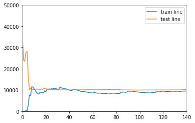
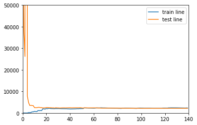
Model learning curve of cubic
drawLearnLinear(poly3,X,y)
This picture is perfect,
- With the increase of training samples, the two lines almost merge, and the generalization ability of the model is very good, which shows that the error of the model is almost the same after training samples to the new samples
- The final error is stable at about 3000, which is much smaller than the previous figure, which also shows that the above model is not fit
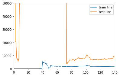
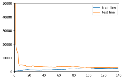
Model learning curve of power 30
drawLearnLinear(poly5,X,y)
- The distance between training samples and test samples is very large and the error of test samples is very unstable, which is large in the sky, over fitting and low in generalization ability
In the practical application process, we are mostly solving the over fitting situation. We use the training data set to train the model, and then we find that the fitting is good, even if the fitting occurs, we don't know. In the high latitude sample space, it is difficult to visualize. So next, we will discuss how to solve the over fitting
Let's print the above models and learn the θ \ theta θ parameter
poly1.get_params()['linear_reg'].coef_
array([ 0. , 186.11946548])
poly2.get_params()['linear_reg'].coef_
array([ 0. , 163.6013378 , -50.05769662])
poly3.get_params()['linear_reg'].coef_
array([ 0. , 2.00832969, -37.03488194, 208.61357956])
poly5.get_params()['linear_reg'].coef_
array([ 3.60460115e+12, -7.50492893e+01,  4.02625575e+02,  7.50064206e+03,
       -5.31983387e+04, -1.89716199e+05,  1.86114685e+06,  1.97519240e+06,
       -3.09333497e+07, -7.12811683e+06,  2.96235084e+08, -3.19140561e+07,
       -1.80711808e+09,  4.60268720e+08,  7.44470660e+09, -2.33671288e+09,
       -2.14435003e+10,  7.02475143e+09,  4.39978121e+10, -1.38712963e+10,
       -6.46641554e+10,  1.85250937e+10,  6.75581331e+10, -1.66255368e+10,
       -4.89684824e+10,  9.62439487e+09,  2.34009853e+10, -3.25078340e+09,
       -6.62797198e+09,  4.87070189e+08,  8.42481030e+08])
It can be found that the absolute value of the learned characteristic coefficient of the over fitted model is very large, so whether we can limit the size of θ \ theta θ to avoid over fitting
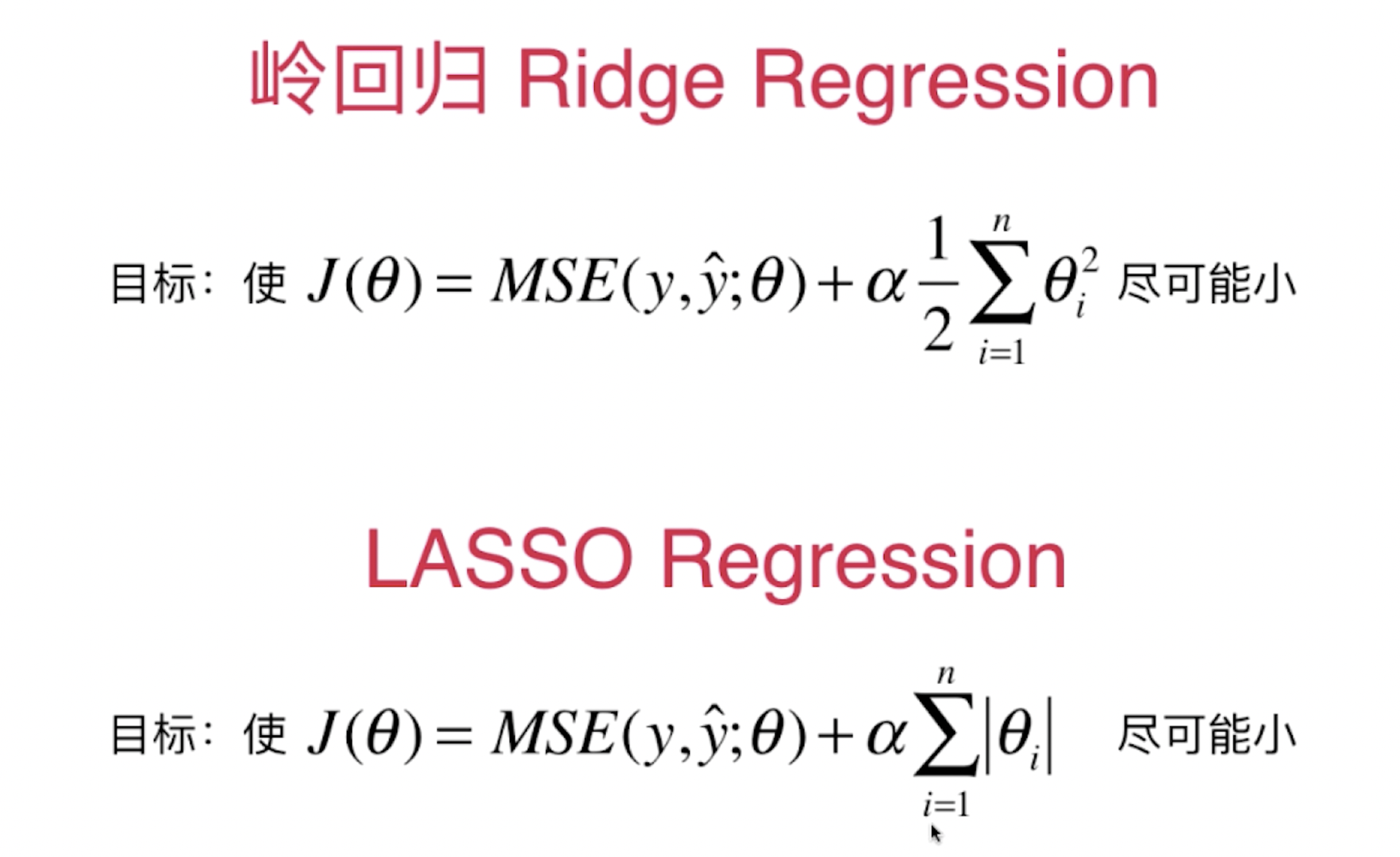
The answer is yes. In the process of minimizing the loss function, we can minimize θ \ theta θ and add a term after the loss function of multiple linear regression
α12∑i=1nθi2
\alpha \frac 1 2 \displaystyle \sum_{i=1}^n \theta_i^2
α21i=1∑nθi2
perhaps
α12∑i=1n∣θi∣
\alpha \frac 1 2 \displaystyle \sum_{i=1}^n |\theta_i|
α21i=1∑n∣θi∣
Then minimize the loss function. Alpha alpha is also a new super parameter. In my understanding, it is used to control the influence proportion of theta theta theta in the loss function
The loss functions of two different regression models are as follows:
Try to use Ridge regression and LASSO regression to solve over fitting
Ridge return
from sklearn.linear_model import Ridge
def ridgeFeatures(degree,alpha):
    return Pipeline([
        ("poly", PolynomialFeatures(degree=degree)),
        ("scaler", StandardScaler()),
        ("linear_reg", Ridge(alpha = alpha))
    ])
If you use the power of 30 power directly, there may be a fitting situation. Let's see the power of Ridge regression
ridge = ridgeFeatures(30,1)

ridge.fit(X_train, y_train)

print("Model prediction accuracy:",ridge.score(X_test,y_test))
Model prediction accuracy: 0.9557567126123063
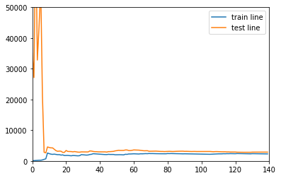
Draw the learning curve again
drawLearnLinear(ridge, X, y)
Something magical happened, R_2. The accuracy of the model is 0.95, and the error and generalization ability are good. This is a training data set containing 30 power of each feature!
LASSO regression
from sklearn.linear_model import Lasso

def lassoFeatures(degree,alpha):
    return Pipeline([
        ("poly", PolynomialFeatures(degree=degree)),
        ("scaler", StandardScaler()),
        ("linear_reg", Lasso(alpha = alpha))
    ])
Use super parameters with possible over fitting
lasso = lassoFeatures(30, 10)
lasso.fit(X_train,y_train)
print("Model prediction accuracy:",lasso.score(X_test,y_test))
Model prediction accuracy: 0.9447394073618249
Draw learning curve
drawLearnLinear(lasso, X, y)
perfect!