1, What is a decision tree

Decision tree is a method of machine learning. The generation algorithms of decision tree include ID3, C4.5 and C5.0. Decision tree is a tree structure, in which each internal node represents a judgment on an attribute, each branch represents the output of a judgment result, and finally each leaf node represents a classification result.

For complex prediction problems, branch nodes are generated by establishing a tree model, which are divided into two (binary tree) or more (multi tree) simpler subsets, which are structurally divided into different subproblems. The process of dividing data sets according to rules is recursive.

With the increasing depth of the tree, the subset of branch nodes becomes smaller and smaller, and the number of problems to be asked is gradually simplified. When the depth of the branch node or the simplicity of the problem meet a certain stop rule, the branch node will stop splitting, which is a top-down stop threshold method; Some decision trees also use bottom-up pruning.

2, ID3 algorithm

1,ID3

ID3 algorithm is a kind of decision tree. It is based on the principle of Occam razor, that is to do more with fewer things as far as possible. ID3 algorithm, i.e. iterative dichotomizer 3, iterative binary tree 3 generation, is a decision tree algorithm invented by Ross Quinlan. The basis of this algorithm is the Okam razor principle mentioned above. The smaller the decision tree, the better the larger the decision tree. Nevertheless, it does not always generate the smallest tree structure, but a heuristic algorithm.

2. Information entropy

The concept of entropy originated from physics. In physics, it is used to measure the disorder degree of a thermodynamic system, while in Informatics, entropy is a measure of uncertainty. In 1948, Shannon introduced information entropy and defined it as the probability of discrete random events. The more ordered a system is, the lower the information entropy is. On the contrary, the more chaotic a system is, the higher its information entropy is. Therefore, information entropy can be considered as a measure of the degree of system ordering.

If the value of a random variable X is:

The probability of each is:

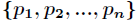
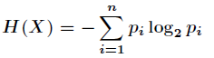
Then the entropy of X is defined as:

For the classification system, category C is a variable, and its value is:

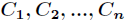
The probability of occurrence of each category is:

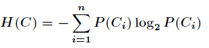
Here n is the total number of categories, and the entropy of the classification system can be expressed as:

3. Information gain

Information gain is aimed at a feature, which is to look at a feature T and the amount of information when the system has it and does not have it. The difference between the two is the amount of information brought to the system by this feature, that is, information gain.

3, Select watermelon

Build the following data sets in excel

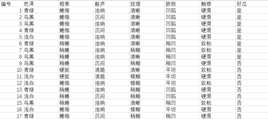
Python code is as follows:

import pandas as pd
import numpy as np
from collections import Counter
from math import log2

#Data acquisition and processing
def getData(filePath):
    data = pd.read_excel(filePath)
    return data

def dataDeal(data):
    dataList = np.array(data).tolist()
    dataSet = [element[1:] for element in dataList]
    return dataSet
    
    #Get property name
def getLabels(data):
    labels = list(data.columns)[1:-1]
    return labels
    
    #Get category tag
def targetClass(dataSet):
    classification = set([element[-1] for element in dataSet])
    return classification
    
    #Mark the branch node as the leaf node, and select the class with the largest number of samples as the class mark
def majorityRule(dataSet):
    mostKind = Counter([element[-1] for element in dataSet]).most_common(1)
    majorityKind = mostKind[0][0]
    return majorityKind
    
    #Calculating information entropy
def infoEntropy(dataSet):
    classColumnCnt = Counter([element[-1] for element in dataSet])
    Ent = 0
    for symbol in classColumnCnt:
        p_k = classColumnCnt[symbol]/len(dataSet)
        Ent = Ent-p_k*log2(p_k)
    return Ent
    
    #Sub dataset construction
def makeAttributeData(dataSet,value,iColumn):
    attributeData = []
    for element in dataSet:
        if element[iColumn]==value:
            row = element[:iColumn]
            row.extend(element[iColumn+1:])
            attributeData.append(row)
    return attributeData
    
    #Calculate information gain
def infoGain(dataSet,iColumn):
    Ent = infoEntropy(dataSet)
    tempGain = 0.0
    attribute = set([element[iColumn] for element in dataSet])
    for value in attribute:
        attributeData = makeAttributeData(dataSet,value,iColumn)
        tempGain = tempGain+len(attributeData)/len(dataSet)*infoEntropy(attributeData)
        Gain = Ent-tempGain
    return Gain
    
    #Select optimal attribute                
def selectOptimalAttribute(dataSet,labels):
    bestGain = 0
    sequence = 0
    for iColumn in range(0,len(labels)):#Ignore the last category column
        Gain = infoGain(dataSet,iColumn)
        if Gain>bestGain:
            bestGain = Gain
            sequence = iColumn
        print(labels[iColumn],Gain)
    return sequence
    
    #Establish decision tree
def createTree(dataSet,labels):
    classification = targetClass(dataSet) #Get category type (collection de duplication)
    if len(classification) == 1:
        return list(classification)[0]
    if len(labels) == 1:
        return majorityRule(dataSet)#Return categories with more sample types
    sequence = selectOptimalAttribute(dataSet,labels)
    print(labels)
    optimalAttribute = labels[sequence]
    del(labels[sequence])
    myTree = {optimalAttribute:{}}
    attribute = set([element[sequence] for element in dataSet])
    for value in attribute:
        
        print(myTree)
        print(value)
        subLabels = labels[:]
        myTree[optimalAttribute][value] =  \
                createTree(makeAttributeData(dataSet,value,sequence),subLabels)
    return myTree
    
def main():
    filePath = 'D:\watermelondata.xls'
    data = getData(filePath)
    dataSet = dataDeal(data)
    labels = getLabels(data)
    myTree = createTree(dataSet,labels)
    return myTree
    
if __name__ == '__main__':
    myTree = main()

The results are as follows:

Color 0.10812516526536531
 Root 0.14267495956679277
 Knock 0.14078143361499584
 Texture 0.3805918973682686
 Umbilical 0.28915878284167895
 Touch 0.006046489176565584
['color and lustre', 'Root', 'stroke ', 'texture', 'Umbilicus', 'Tactile sensation']
{'texture': {}}
Slightly paste
 Color 0.3219280948873623
 Root 0.07290559532005603
 Knock 0.3219280948873623
 Umbilical 0.17095059445466865
 Touch 0.7219280948873623
['color and lustre', 'Root', 'stroke ', 'Umbilicus', 'Tactile sensation']
{'Tactile sensation': {}}
Hard slip
{'Tactile sensation': {'Hard slip': 'no'}}
Soft sticky
{'texture': {'Slightly paste': {'Tactile sensation': {'Hard slip': 'no', 'Soft sticky': 'yes'}}}}
clear
 Color 0.04306839587828004
 Root 0.45810589515712374
 Knock 0.33085622540971754
 Umbilical 0.45810589515712374
 Touch 0.45810589515712374
['color and lustre', 'Root', 'stroke ', 'Umbilicus', 'Tactile sensation']
{'Root': {}}
Stiff
{'Root': {'Stiff': 'no'}}
Curl up
{'Root': {'Stiff': 'no', 'Curl up': 'yes'}}
Slightly curled
 Color 0.2516291673878229
 Knock 0.0
 Umbilical 0.0
 Touch 0.2516291673878229
['color and lustre', 'stroke ', 'Umbilicus', 'Tactile sensation']
{'color and lustre': {}}
dark green
{'color and lustre': {'dark green': 'yes'}}
Black
 Knock 0.0
 Umbilical 0.0
 Tactile 1.0
['stroke ', 'Umbilicus', 'Tactile sensation']
{'Tactile sensation': {}}
Hard slip
{'Tactile sensation': {'Hard slip': 'yes'}}
Soft sticky
{'texture': {'Slightly paste': {'Tactile sensation': {'Hard slip': 'no', 'Soft sticky': 'yes'}}, 'clear': {'Root': {'Stiff': 'no', 'Curl up': 'yes', 'Slightly curled': {'color and lustre': {'dark green': 'yes', 'Black': {'Tactile sensation': {'Hard slip': 'yes', 'Soft sticky': 'no'}}}}}}}}
vague

4, The algorithm codes of ID3, C4.5 and CART are implemented for watermelon data set with SK learn library

1.ID3

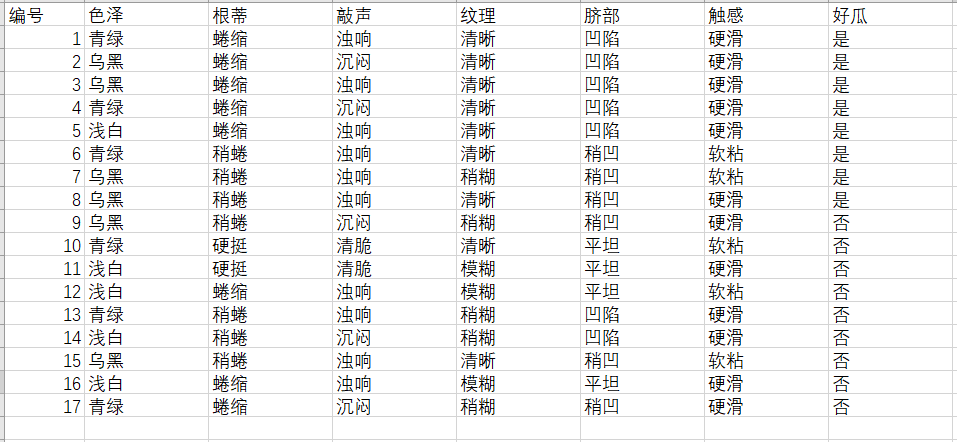
Create a dataset as shown in the figure

import pandas as pd
import graphviz 
from sklearn.model_selection import train_test_split
from sklearn import tree

f = open('D:\watermelondata.csv',encoding='utf-8')
data = pd.read_csv(f)

x = data[["color and lustre","Root","stroke ","texture","Umbilicus","Tactile sensation"]].copy()
y = data['Good melon'].copy()
print(data)
#Numeric eigenvalues
x = x.copy()
for i in ["color and lustre","Root","stroke ","texture","Umbilicus","Tactile sensation"]:
    for j in range(len(x)):
        if(x[i][j] == "dark green" or x[i][j] == "Curl up" or data[i][j] == "Turbid sound" \
           or x[i][j] == "clear" or x[i][j] == "sunken" or x[i][j] == "Hard slip"):
            x[i][j] = 1
        elif(x[i][j] == "Black" or x[i][j] == "Slightly curled" or data[i][j] == "Dull" \
           or x[i][j] == "Slightly paste" or x[i][j] == "Slightly concave" or x[i][j] == "Soft sticky"):
            x[i][j] = 2
        else:
            x[i][j] = 3
            
y = y.copy()
for i in range(len(y)):
    if(y[i] == "yes"):
        y[i] = int(1)
    else:
        y[i] = int(-1) 
#You need to convert the data x and y into a good format and the data frame dataframe, otherwise the format will report an error
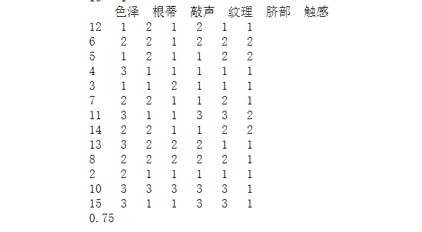
x = pd.DataFrame(x).astype(int)
y = pd.DataFrame(y).astype(int)
print(x)
print(y)

x_train, x_test, y_train, y_test = train_test_split(x,y,test_size=0.2)
print(x_train)

#Decision tree learning
clf = tree.DecisionTreeClassifier(criterion="entropy")                    #instantiation  
clf = clf.fit(x_train, y_train) 
score = clf.score(x_test, y_test)
print(score)

Select "root", "knock", "texture", "navel", "touch" for training

2.C4.5

(1) Defects of ID3

For ID3 algorithm, it has the following problems:

• Attributes with multiple values are easier to make the data more pure and have greater information gain;
• The training result is a huge and shallow tree, which is unreasonable.

C4.5 algorithm can suppress the above shortcomings of ID3.

(2) C4.5 algorithm

C4.5 algorithm is an algorithm developed by Ross Quinlan to generate decision tree. The algorithm is based on Ross
An extension of the ID3 algorithm previously developed by Quinlan. The decision tree generated by C4.5 algorithm can be used for classification purposes, so the algorithm can also be used for statistical classification. It performs feature selection through information gain ratio.

(3) Information gain rate

If a certain condition is extremely strict, for example, a student knows the answers of all topics in advance, then taking the serial number of topics as the condition, there is no uncertainty, so the maximum information gain can be obtained. But this condition is meaningless. If the teacher changes a test paper, all the answers will be invalid.

The information gain rate adds a penalty term based on the information gain. The penalty term is the inherent value of the feature and is designed to avoid the above situation.

Write gr(X,Y). It is defined as the information gain divided by the intrinsic value of the characteristic, as follows

Continue to take the single choice question as an example. After analyzing the length characteristics of the topic, the information gain g(X,Y) is 2bit, and the penalty term H (Y) = -0.1log0.1-0.1log0.1-0.8*log0.8=0.92

The information gain rate is 0.4 / 0.92 = 43%, of which the information gain rate is 43%.

3.CART operator

(1)CART

CART is a binary tree. Each split will produce two child nodes. CART tree is divided into classification tree and regression tree.

The classification tree mainly aims at the target scalar as the classification variable, such as predicting whether an animal is a mammal.

The regression tree is used to predict the age of an animal when the target variable is a continuous value.

If it is a classification tree, the split attribute that can minimize the GINI value of the split node will be selected;

If it is a regression tree, select the splitting attribute that can minimize the sample variance of two nodes. CART, like other decision tree algorithms, needs pruning to prevent the algorithm from over fitting, so as to ensure the generalization performance of the algorithm.

(2) Gini index

CART decision tree algorithm uses Gini index to select partition attributes. Gini index is defined as:

          Gini(D) = ∑k=1 ∑k'≠1 pk·pk' = 1- ∑k=1  pk·pk

Gini index can be understood as follows: the probability that two samples are randomly selected from data set D and their category labels are inconsistent. The smaller Gini(D), the higher the purity.

Definition of Gini index for attribute a:

      Gain_index(D,a) = ∑v=1 |Dv|/|D|·Gini(Dv)

The Gini index is used to select the optimal partition attribute, that is, the attribute that minimizes the Gini index after partition is selected as the optimal partition attribute.

summary

The main purpose of this experiment is to understand and be familiar with a simple machine learning with ID3 algorithm without SK learn and with SK learn. At the same time, C4.5 algorithm and CART algorithm are understood.

Reference articles

https://blog.csdn.net/weixin_56102526/article/details/120987844?spm=1001.2014.3001.5501
https://blog.csdn.net/qq_45659777/article/details/120960616?spm=1001.2014.3001.5501