1, Introduction
Decision tree is a classification algorithm based on tree structure. We hope to learn a model (i.e. decision tree) from a given training data set and use the model to classify new samples. The decision tree can intuitively show the classification process and results. Once the model is built successfully, the classification efficiency of new samples is also quite high.
The most classical decision tree algorithms are ID3, C4.5 and CART. ID3 algorithm was first proposed. It can deal with the classification of discrete attribute samples. C4.5 and CART algorithms can deal with more complex classification problems. This paper focuses on ID3 algorithm
2, Build a model based on the scene of buying watermelon
1. Introduce examples
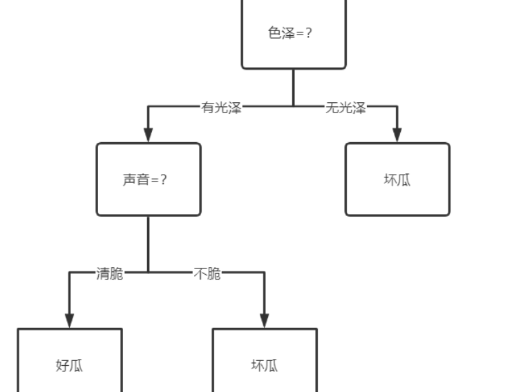
For example: when I buy watermelon in summer, I usually choose the one with shiny skin (fresh), and then take a pat to choose the one with crisp sound (mature), so I may have more good melons. So here's my decision tree for picking watermelon
So how do we choose the attributes of the optimal partition
Through learning, we can know
2. Use the information gain to select the optimal partition attribute
The sample has multiple attributes. Which sample should be selected first to divide the data set?
The principle is that with the continuous division, we hope that the samples contained in the branch nodes of the decision tree belong to the same classification as much as possible, that is, the "purity" is getting higher and higher. Let's learn about "information entropy" and "information gain".
Two concepts are introduced below
information entropy
The proportion of class k samples in sample set D (k=1,2,...,|Y|). |Y| is the number of sample classifications, then the information entropy of D is:
The smaller the value of Ent(D), the higher the purity of D. Intuitively understand: suppose that the sample set has two classifications, the proportion of each type of sample is 1 / 2, Ent(D)=1; There is only one classification, Ent(D) = 0. Obviously, the purity of the latter is higher than that of the former.
In the watermelon sample set, there are 17 samples, including 8 positive samples and 9 negative samples. The information entropy of the sample set is:
information gain
The "information gain" obtained by dividing the sample set D with attribute a is calculated by subtracting the product of the information entropy of each branch of attribute a and the weight (the number of samples of this branch divided by the total number of samples) from the total information entropy of the sample set. Generally, the greater the information gain, the greater the "purity improvement" obtained by dividing the sample set D with attribute a. Therefore, the attribute with the largest information gain is preferentially selected for division. If attribute a has V possible values, the information gain of attribute a is:
In the watermelon sample set, taking the attribute "color" as an example, it has three values {cyan, ebony and light white}. There are 6 samples in the corresponding subset (color = cyan), including 3 positive and negative samples, 6 samples in (color = ebony), 4 positive samples and 2 negative samples, 5 samples in (color = light white), 1 positive sample and 4 negative samples.
Just like this, we calculate the information gain of several other attributes, select the attribute with the largest information gain as the root node for division, and then further divide each branch.
Now let's take this first step
3. The code realizes the calculation information gain selection division.
#Import data and related packages
import pandas as pd
import numpy as np
from collections import Counter
from math import log2
fr = open(r'D:\baidu\watermalon.txt',encoding="utf-8")
listWm = [inst.strip().split(' ') for inst in fr.readlines()]
print(listWm)
See the following data
Calculate the information entropy according to what you have learned before
def calcShannonEnt(dataSet):
    numEntries = len(dataSet)  # Number of samples
    labelCounts = {}
    for featVec in dataSet:  # Traverse each sample
        currentLabel = featVec[-1]  # Category of the current sample
        if currentLabel not in labelCounts.keys():  # Generate category dictionary
            labelCounts[currentLabel] = 0
        labelCounts[currentLabel] += 1
    shannonEnt = 0.0
    for key in labelCounts:  # Calculating information entropy
        prob = float(labelCounts[key]) / numEntries
        shannonEnt = shannonEnt - prob * log(prob, 2)
    return shannonEnt
print(calcShannonEnt(listWm))
First, define a function to divide the data set
# Divide the dataset, axis: divide by the first attribute, value: the attribute value corresponding to the subset to be returned
def splitDataSet(dataSet, axis, value):
    retDataSet = []
    featVec = []
    for featVec in dataSet:
        if featVec[axis] == value:
            reducedFeatVec = featVec[:axis]
            reducedFeatVec.extend(featVec[axis + 1:])
            retDataSet.append(reducedFeatVec)
    return retDataSet
Then the most appropriate divided attribute is selected by calculating the information gain of the current attribute
# Select the best data set division method
def chooseBestFeatureToSplit(dataSet):
    numFeatures = len(dataSet[0]) - 1  # Number of attributes
    baseEntropy = calcShannonEnt(dataSet)
    bestInfoGain = 0.0
    bestFeature = -1
    for i in range(numFeatures):  # Technical information gain for each attribute
        featList = [example[i] for example in dataSet]
        uniqueVals = set(featList)  # Value collection of this attribute
        newEntropy = 0.0
        for value in uniqueVals: # Calculate the information gain for each value
            subDataSet = splitDataSet(dataSet, i, value)
            prob = len(subDataSet) / float(len(dataSet))
            newEntropy += prob * calcShannonEnt(subDataSet)
        infoGain = baseEntropy - newEntropy
        if (infoGain > bestInfoGain):  # Select the attribute with the largest information gain
            bestInfoGain = infoGain
            bestFeature = i
    return bestFeature
print(chooseBestFeatureToSplit(listWm))
The output is three, that is, the column with sequence number three should be selected first as the split attribute
4. Recursive construction of decision tree
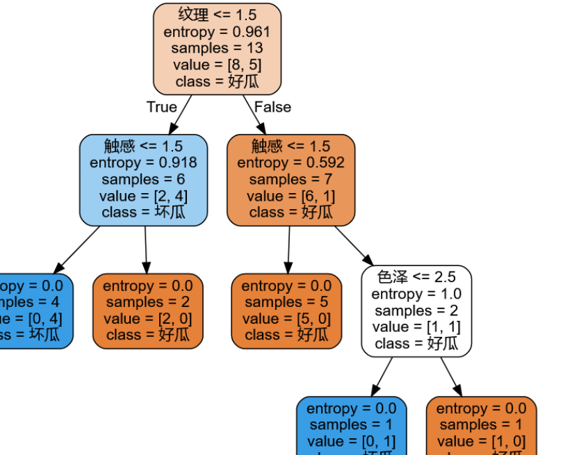
Usually, a decision tree contains a root node, several branch nodes and several leaf nodes. The leaf node corresponds to the decision result (such as good melon or bad melon), the root node and branch node correspond to an attribute test (such as color =?), and the sample set contained in each node is divided into child nodes according to the result of attribute test.
In the previous section, the optimal partition attribute we selected for the whole training set is the root node. After the first partition, the data is passed down to the next node of the tree branch, and then we can partition the data again. Building the decision tree is a recursive process, and the condition for the end of recursion is that all attributes are traversed, Or all samples under each branch belong to the same class.
In another case, when a node is divided, the corresponding attribute values of the node are the same, but the sample categories are different. At this time, the current node is marked as a leaf node and its category is set as the category with more samples. For example, when a branch is divided, there are three samples in the node, and the optimal division attribute is color, and the value of color is only one "light white", and there are two good melons in the three samples. At this time, we mark this node as the leaf node "good melon".
import operator  # This line is added at the top of the file

# The category with the most occurrences is returned by sorting
def majorityCnt(classList):
    classCount = {}
    for vote in classList:
        if vote not in classCount.keys(): classCount[vote] = 0
        classCount[vote] += 1
    sortedClassCount = sorted(classCount.iteritems(),
                              key=operator.itemgetter(1), reverse=True)
    return sortedClassCount[0][0]


# Recursive construction of decision tree
def createTree(dataSet, labels):
    classList = [example[-1] for example in dataSet]  # Category vector
    if classList.count(classList[0]) == len(classList):  # If there is only one category, return
        return classList[0]
    if len(dataSet[0]) == 1:  # If all features are traversed, the category with the most occurrences is returned
        return majorityCnt(classList)
    bestFeat = chooseBestFeatureToSplit(dataSet)  # Index of optimal partition attribute
    bestFeatLabel = labels[bestFeat]  # Label of optimal partition attribute
    myTree = {bestFeatLabel: {}}
    del (labels[bestFeat])  # The selected features are no longer involved in classification
    featValues = [example[bestFeat] for example in dataSet]
    uniqueValue = set(featValues)  # All possible values of this attribute, that is, the branch of the node
    for value in uniqueValue:  # For each branch, the tree is constructed recursively
        subLabels = labels[:]
        myTree[bestFeatLabel][value] = createTree(
            splitDataSet(dataSet, bestFeat, value), subLabels)
    return myTree
Finally, test the algorithm with data,. Because the generated tree is represented in Chinese, the json.dumps() method is used to print the results. If it does not contain Chinese, print directly.
# -*- coding: cp936 -*-
import trees
import json

fr = open(r'C:\Python27\py\DecisionTree\watermalon.txt')

listWm = [inst.strip().split('\t') for inst in fr.readlines()]
labels = ['color and lustre', 'Root', 'stroke ', 'texture', 'Umbilicus', 'Tactile sensation']
Trees = trees.createTree(listWm, labels)

print json.dumps(Trees, encoding="cp936", ensure_ascii=False)
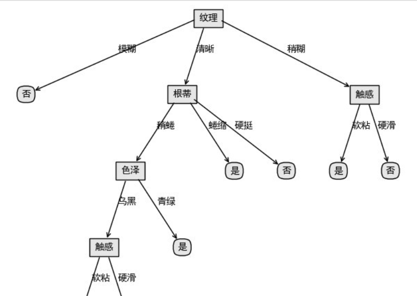
give the result as follows
{"texture": {"fuzzy": "no", "clear": {"root": {"slightly curled": {"color": {"dark": {"touch": {"soft stick": "no", "hard slip": "yes"}}, "Turquoise": "yes"}}, "curled up": "yes", "hard": "no"}}, "slightly paste": {"touch": {"soft stick": "yes", "hard slip": "no"}}}
5. Use Matplotlib to draw the decision tree
The decision tree in dictionary form is still difficult to understand. Next, we draw the decision tree by using the annotate module of Matplotlib library, and we can intuitively see the structure of the decision tree
# -*- coding: cp936 -*-
import matplotlib.pyplot as plt

# Set the border shape, margin and transparency of decision and leaf nodes, as well as the shape of arrows
decisionNode = dict(boxstyle="square,pad=0.5", fc="0.9")
leafNode = dict(boxstyle="round4, pad=0.5", fc="0.9")
arrow_args = dict(arrowstyle="<-", connectionstyle="arc3", shrinkA=0,
                  shrinkB=16)


def plotNode(nodeTxt, centerPt, parentPt, nodeType):
    createPlot.ax1.annotate(unicode(nodeTxt, 'cp936'), xy=parentPt,
                            xycoords='axes fraction',
                            xytext=centerPt, textcoords='axes fraction',
                            va="top", ha="center", bbox=nodeType,
                            arrowprops=arrow_args)


def getNumLeafs(myTree):
    numLeafs = 0
    firstStr = myTree.keys()[0]
    secondDict = myTree[firstStr]
    for key in secondDict.keys():
        if type(secondDict[key]).__name__ == 'dict':
            numLeafs += getNumLeafs(secondDict[key])
        else:
            numLeafs += 1
    return numLeafs


def getTreeDepth(myTree):
    maxDepth = 0
    firstStr = myTree.keys()[0]
    secondDict = myTree[firstStr]
    for key in secondDict.keys():
        if type(secondDict[key]).__name__ == 'dict':
            thisDepth = 1 + getTreeDepth(secondDict[key])
        else:
            thisDepth = 1
        if thisDepth > maxDepth: maxDepth = thisDepth
    return maxDepth


def plotMidText(cntrPt, parentPt, txtString):
    xMid = (parentPt[0] - cntrPt[0]) / 2.0 + cntrPt[0]
    yMid = (parentPt[1] - cntrPt[1]) / 2.0 + cntrPt[1]
    createPlot.ax1.text(xMid, yMid, unicode(txtString, 'cp936'))


def plotTree(myTree, parentPt, nodeTxt):
    numLeafs = getNumLeafs(myTree)
    depth = getTreeDepth(myTree)
    firstStr = myTree.keys()[0]
    cntrPt = (plotTree.xOff + (1.0 + float(numLeafs)) / 2.0 / plotTree.totalW,
              plotTree.yOff)
    plotMidText(cntrPt, parentPt, nodeTxt)
    plotNode(firstStr, cntrPt, parentPt, decisionNode)
    secondDict = myTree[firstStr]
    plotTree.yOff = plotTree.yOff - 1.0 / plotTree.totalD
    for key in secondDict.keys():
        if type(secondDict[key]).__name__ == 'dict':
            plotTree(secondDict[key], cntrPt, str(key))
        else:
            plotTree.xOff = plotTree.xOff + 1.0 / plotTree.totalW
            plotNode(secondDict[key], (plotTree.xOff, plotTree.yOff),
                     cntrPt, leafNode)
            plotMidText((plotTree.xOff, plotTree.yOff), cntrPt, str(key))
    plotTree.yOff = plotTree.yOff + 1.0 / plotTree.totalD


def createPlot(inTree):
    fig = plt.figure(1, facecolor='white')
    fig.clf()
    axprops = dict(xticks=[], yticks=[])
    createPlot.ax1 = plt.subplot(111, frameon=False, **axprops)
    plotTree.totalW = float(getNumLeafs(inTree))
    plotTree.totalD = float(getTreeDepth(inTree))
    plotTree.xOff = -0.5 / plotTree.totalW
    plotTree.yOff = 1.0
    plotTree(inTree, (0.5, 1.0), '')
    plt.show()
# -*- coding: cp936 -*-
import trees
import treePlotter
import json

fr = open(r'C:\Python27\py\DecisionTree\watermalon.txt')

listWm = [inst.strip().split('\t') for inst in fr.readlines()]
labels = ['color and lustre', 'Root', 'stroke ', 'texture', 'Umbilicus', 'Tactile sensation']
Trees = trees.createTree(listWm, labels)

print json.dumps(Trees, encoding="cp936", ensure_ascii=False)

treePlotter.createPlot(Trees)
3, Algorithm code implementation of ID3, C4.5 and CART (using Sklearn)
1. Import related libraries
#Import related libraries
import pandas as pd
import graphviz
from sklearn.model_selection import train_test_split
from sklearn import tree

f = open('watermelon2.csv','r')
data = pd.read_csv(f)

x = data[["color and lustre","Root","stroke ","texture","Umbilicus","Tactile sensation"]].copy()
y = data['Good melon'].copy()
print(data)
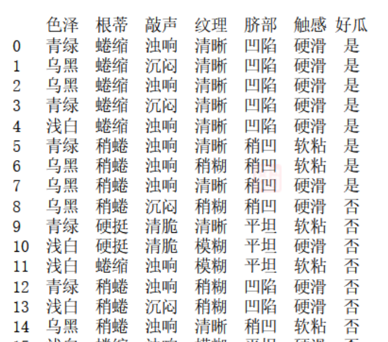
The characteristic function is digitized and the decision tree is learned. Finally, the obtained decision tree is drawn
#Numeric eigenvalues
x = x.copy()
for i in ["color and lustre","Root","stroke ","texture","Umbilicus","Tactile sensation"]:
for j in range(len(x)):
if(x[i][j] == "dark green" or x[i][j] == "Curl up" or data[i][j] == "Turbid sound" \
or x[i][j] == "clear" or x[i][j] == "sunken" or x[i][j] == "Hard slip"):
x[i][j] = 1
elif(x[i][j] == "Black" or x[i][j] == "Slightly curled" or data[i][j] == "Dull" \
or x[i][j] == "Slightly paste" or x[i][j] == "Slightly concave" or x[i][j] == "Soft sticky"):
x[i][j] = 2
else:
x[i][j] = 3
y = y.copy()
for i in range(len(y)):
if(y[i] == "yes"):
y[i] = int(1)
else:
y[i] = int(-1)
#You need to convert the data x and y into a good format and the data frame dataframe, otherwise the format will report an error
x = pd.DataFrame(x).astype(int)
y = pd.DataFrame(y).astype(int)
print(x)
print(y)
x_train, x_test, y_train, y_test = train_test_split(x,y,test_size=0.2)
print(x_train)
#Decision tree learning
clf = tree.DecisionTreeClassifier(criterion="entropy") #instantiation
clf = clf.fit(x_train, y_train)
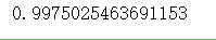
score = clf.score(x_test, y_test)
print(score)
# Plus graphviz 2.38 absolute path
import os
os.environ["PATH"] += os.pathsep + 'C:/Program Files (x86)/Graphviz2.38/bin'
feature_name = ["color and lustre","Root","stroke ","texture","Umbilicus","Tactile sensation"]
dot_data = tree.export_graphviz(clf ,feature_names= feature_name,class_names=["Good melon","Bad melon"],filled=True,rounded=True,out_file =None)
graph = graphviz.Source(dot_data)
4, C4.5 algorithm
1.C4.5 algorithm Introduction
C4.5 algorithm is a classical algorithm used to generate decision tree. It is an extension and optimization of ID3 algorithm. C4.5 algorithm mainly makes the following improvements to ID3 algorithm:
(1) selecting split attributes through information gain rate overcomes the tendency to select attributes with multiple attribute values through information gain in ID3 algorithm As a split attribute;
(2) it can handle discrete and continuous attribute types, that is, discrete continuous attributes;
(3) pruning after constructing the decision tree;
(4) it can process training data with missing attribute values.
2. Split attribute selection
- Information gain rate
The criterion of split attribute selection is the fundamental difference between decision tree algorithms. Different from ID3 algorithm, C4.5 algorithm selects splitting attributes through information gain rate.
split information of attribute A:
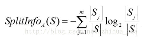
Among them, the training data set S is divided into m sub data sets through the attribute value of attribute A, | Sj | represents the number of samples in the j-th sub data set, and | S | represents the total number of samples in the data set before division.
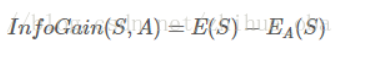
information gain of sample set after splitting through attribute A:
Information gain rate of sample set after splitting through attribute A:
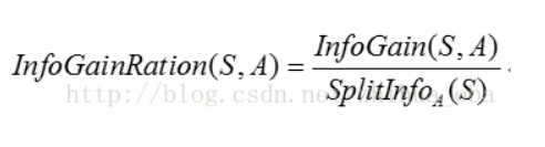
When constructing the decision tree through C4.5 algorithm, the attribute with the largest information gain rate is the split attribute of the current node. With recursive calculation, the information gain rate of the calculated attribute will become smaller and smaller. In the later stage, the attribute with relatively large information gain rate will be selected as the split attribute.
3. Analysis of advantages and disadvantages of C4.5 algorithm
advantage:
(1) The split attribute is selected by the information gain rate, which overcomes the deficiency that ID3 algorithm tends to select attributes with multiple attribute values as split attributes through information gain;
(2) It can handle discrete and continuous attribute types, that is, discrete continuous attributes;
(3) Pruning after constructing the decision tree;
(4) It can process training data with missing attribute values.
Disadvantages:
(1) The computational efficiency of the algorithm is low, especially for the training samples with continuous attribute values.
(2) The algorithm does not consider the correlation between conditional attributes when selecting split attributes, and only calculates the expected information between each conditional attribute and decision attribute in the data set, which may affect the correctness of attribute selection.
4.python implementation
## Information gain rate
def chooseBestFeatureToSplit_4(dataSet, labels):
    """
    The best data set partition feature is selected and calculated according to the information gain value
    :param dataSet:
    :return:
    """
    # Get the total number of eigenvalues of the data
    numFeatures = len(dataSet[0]) - 1

    # Calculate the basic information entropy
    baseEntropy = calcShannonEnt(dataSet)

    # The gain of basic information is 0.0
    bestInfoGain = 0.0

    # Best eigenvalue
    bestFeature = -1

    # Calculate the information entropy of each eigenvalue
    for i in range(numFeatures):
        # Get a list of all current eigenvalues in the dataset
        featList = [example[i] for example in dataSet]

        # Make the current feature unique, that is, how many kinds of current feature values are there
        uniqueVals = set(featList)

        # The new entropy represents the entropy of the current eigenvalue
        newEntropy = 0.0

        # Possibility of traversing existing features
        for value in uniqueVals:
            # At the current feature position of all data sets, find the set whose feature value is equal to the current value
            subDataSet = splitDataSet(dataSet=dataSet, axis=i, value=value)

            # Calculate the weight
            prob = len(subDataSet) / float(len(dataSet))

            # Calculate the entropy of the current eigenvalue
            newEntropy += prob * calcShannonEnt(subDataSet)

        # Calculate the "information gain"
        infoGain = baseEntropy - newEntropy
        infoGain = infoGain/newEntropy

        #print('current characteristic value: '+ labels[i] +', corresponding information gain value: '+ str(infoGain)+"i equals" + str(i))

        #If the current information gain is greater than the original
        if infoGain > bestInfoGain:
            # Best information gain
            bestInfoGain = infoGain
            # The new best eigenvalue is used to divide
            bestFeature = i

    #print('features with maximum information gain: '+ labels[bestFeature])
    return bestFeature
5, CART algorithm
1. Understanding of cart algorithm
Classification And Regression Tree, i.e. Classification And Regression Tree algorithm, referred to as CART algorithm, is an implementation of decision tree. Generally, there are three main implementations of decision tree, namely ID3 algorithm, CART algorithm and C4.5 algorithm.
CART algorithm is a binary recursive segmentation technology, which divides the current sample into two sub samples, so that each non leaf node has two branches. Therefore, the decision tree generated by CART algorithm is a binary tree with simple structure. Because CART algorithm is a binary tree, it can only be "yes" or "no" in each step of decision-making. Even if a feature has multiple values, it also divides the data into two parts. The CART algorithm is mainly divided into two steps
(1) Recursive partition of samples for tree building process
(2) Pruning with validation data
2. Principle of cart algorithm
As mentioned above, the CART algorithm is divided into two processes. The first process recursively establishes a binary tree. How is it divided?
Let x1,x2... xn represent n attributes of a single sample, and y represents the category. CART algorithm divides the n-dimensional space into non overlapping rectangles by recursion. The division steps are roughly as follows
(1) Select an independent variable xi, and then select a value vi of xi. vi divides the n-dimensional space into two parts. All points of one part meet xi < = vi, and all points of the other part meet xi > vi. for discontinuous variables, there are only two values of attribute values, that is, they are equal to or not equal to the value.
(2) Recursive processing, re select an attribute from the above two parts according to step (1) and continue to divide until the whole n-dimensional space is divided. There is A problem in the division. What criteria is it divided according to? For A variable attribute, its partition point is the midpoint of A pair of continuous variable attribute values. Assuming that an attribute of A set of M samples has an m-continuous value, there will be m-1 splitting points, and each splitting point is the mean of two adjacent continuous values. The division of each attribute is sorted according to the amount of impurities that can be reduced, and the reduction of impurities is defined as the sum of the impurities before division minus the proportion of impurity mass division of each node after division. The Gini index is commonly used in impurity measurement methods. Assuming that A sample has class C, the Gini impurity of A node A can be defined as
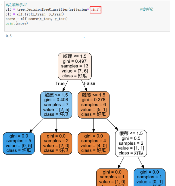
3.python is implemented with sklearn
You only need to change the value of the parameter criterion of the DecisionTreeClassifier function to gini:
6, Summary
Decision tree actually classifies objects by their characteristics. Different people have different classification methods. The results of each method may be different, but it has its reason, but what we have to do is to write the one that can best meet the requirements.
Learning reference:
https://blog.csdn.net/weixin_46129506/article/details/120987574