Preface

tensorflow has an official attitude estimation project. This input is a little different from that of openpost. Here is a single person model output analysis scheme.

International practice, see blog:

Blog: using TensorFlow.js to realize real-time human posture detection on the browser

IOS code of posnet in tensorflow

analysis

Do not download Official overview website To download the postent, person, mobile, V1, float.tflite model, you need to download the postent, mobile, V1, 100, multi, KPT, stripped.tflite model on the IOS side. At the end of the article, you need to put the download address of the network disk.

Read model

Load the necessary kit first:

import numpy as np
import tensorflow as tf
import cv2 as cv
import matplotlib.pyplot as plt
import time

Using tflite to load model files

model = tf.lite.Interpreter('posenet_mobilenet_v1_100_257x257_multi_kpt_stripped.tflite')
model.allocate_tensors()
input_details = model.get_input_details()
output_details = model.get_output_details()

See what the input and output are

print(input_details)
print(output_details)
'''
[{'name': 'sub_2', 'index': 93, 'shape': array([  1, 257, 257,   3], dtype=int32), 'dtype': <class 'numpy.float32'>, 'quantization': (0.0, 0)}]
[{'name': 'MobilenetV1/heatmap_2/BiasAdd', 'index': 87, 'shape': array([ 1,  9,  9, 17], dtype=int32), 'dtype': <class 'numpy.float32'>, 'quantization': (0.0, 0)}, {'name': 'MobilenetV1/offset_2/BiasAdd', 'index': 90, 'shape': array([ 1,  9,  9, 34], dtype=int32), 'dtype': <class 'numpy.float32'>, 'quantization': (0.0, 0)}, {'name': 'MobilenetV1/displacement_fwd_2/BiasAdd', 'index': 84, 'shape': array([ 1,  9,  9, 32], dtype=int32), 'dtype': <class 'numpy.float32'>, 'quantization': (0.0, 0)}, {'name': 'MobilenetV1/displacement_bwd_2/BiasAdd', 'index': 81, 'shape': array([ 1,  9,  9, 32], dtype=int32), 'dtype': <class 'numpy.float32'>, 'quantization': (0.0, 0)}]
'''

It is easy to see that the input is a (257257) size color image.

The output is more cumbersome. There are two parts: (9,9,17) is called heatmap's heat map; (9,9,34) is called offset's offset map. In fact, if you think about it, you can also know that the heat map is used to locate the approximate position of the joint, and the offset map is used for further correction. Next, we will analyze how to use these two outputs to locate the joint position step by step.

Input image inference

You have to resize the image and then throw it in, but tensorflowjs doesn't use the resize method, I haven't tried it yet.

img = cv.imread('../../photo/1.jpeg')
input_img = tf.reshape(tf.image.resize(img, [257,257]), [1,257,257,3])
floating_model = input_details[0]['dtype'] == np.float32
if floating_model:
    input_img = (np.float32(input_img) - 127.5) / 127.5
model.set_tensor(input_details[0]['index'], input_img)
start = time.time()
model.invoke()
print('time:',time.time()-start)
output_data =  model.get_tensor(output_details[0]['index'])
offset_data = model.get_tensor(output_details[1]['index'])
heatmaps = np.squeeze(output_data)
offsets = np.squeeze(offset_data)
print("output shape: {}".format(output_data.shape))
'''
time: 0.12212681770324707
output shape: (1, 9, 9, 17)
'''

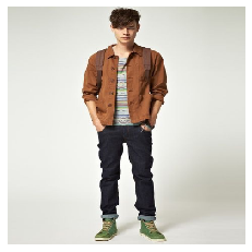
Visualized transformed graph

show_img = np.squeeze((input_img.copy()*127.5+127.5)/255.0)[:,:,::-1]
show_img = np.array(show_img*255,np.uint8)
plt.imshow(show_img)
plt.axis('off')

Analytical output

In a word, the principle is summarized as follows: the heat map divides the image into grids, and the score of each grid represents the probability of the current joint near the grid point; the offset map represents the offset of xy coordinates relative to the grid point.

Suppose to extract the coordinate position of the second joint:

• Get the most likely grid points first:

  i=1
  joint_heatmap = heatmaps[...,i]
  max_val_pos = np.squeeze(np.argwhere(joint_heatmap==np.max(joint_heatmap)))
  remap_pos = np.array(max_val_pos/8*257,dtype=np.int32)
  

• Add the offset. The first 1-17 is the x-coordinate offset, and the last 18-34 is the y-coordinate offset

  refine_pos = np.zeros((2),dtype=int)
  refine_pos[0] = int(remap_pos[0] + offsets[max_val_pos[0],max_val_pos[1],i])
  refine_pos[1] = int(remap_pos[1] + offsets[max_val_pos[0],max_val_pos[1],i+heatmaps.shape[-1]])
  

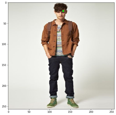
Visualization

show_img = np.squeeze((input_img.copy()*127.5+127.5)/255.0)[:,:,::-1]
show_img = np.array(show_img*255,np.uint8)
plt.figure(figsize=(8,8))
plt.imshow(cv.circle(show_img,(refine_pos[1],refine_pos[0]),2,(0,255,0),-1))

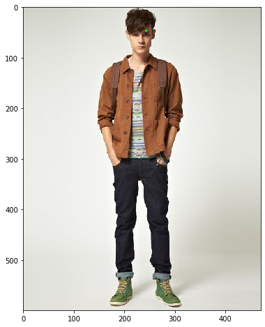
Mapping original graph

Because the above is the coordinate after resizing the original image by (257257), remap it according to the scale factor of the original image

ratio_x = img.shape[0]/257
ratio_y = img.shape[1]/257
refine_pos[0]=refine_pos[0]*ratio_x
refine_pos[1]=refine_pos[1]*ratio_y

visualization

show_img1 = img[:,:,::-1]
plt.figure(figsize=(8,8))
plt.imshow(cv.circle(show_img1.copy(),(refine_pos[1],refine_pos[0]),2,(0,255,0),-1))

Encapsulation function

The above is to extract a single joint, which is written as a function to extract the coordinates of all joints

def parse_output(heatmap_data,offset_data):
    joint_num = heatmap_data.shape[-1]
    pose_kps = np.zeros((joint_num,2),np.uint8)
    for i in range(heatmap_data.shape[-1]):
        joint_heatmap = heatmap_data[...,i]
        max_val_pos = np.squeeze(np.argwhere(joint_heatmap==np.max(joint_heatmap)))
        remap_pos = np.array(max_val_pos/8*257,dtype=np.int32)
        pose_kps[i,0] = int(remap_pos[0] + offset_data[max_val_pos[0],max_val_pos[1],i])
        pose_kps[i,1] = int(remap_pos[1] + offset_data[max_val_pos[0],max_val_pos[1],i+joint_num])
    return pose_kps

It's easy to draw functions

def draw_kps(show_img,kps):
    for i in range(kps.shape[0]):
        cv.circle(show_img,(kps[i,1],kps[i,0]),2,(0,255,0),-1)
    return show_img

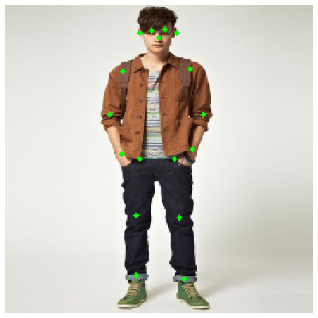
Draw it and look at it

kps = parse_output(heatmaps,offsets)
plt.figure(figsize=(8,8))
plt.imshow(draw_kps(show_img.copy(),kps))
plt.axis('off')

Epilogue

Model file: link: https://pan.baidu.com/s/1herkffz28yvampfqdeaxw password: 5tuw

Blog Code: link: https://pan.baidu.com/s/1Y7WXfQ4WC9QyOGkkN2-kUQ password: ono0