What is NUMA?
NUMA (non uniform memory access) refers to Non-Uniform Memory Access. In order to better explain what NUMA is, we need to talk about the background of NuMA's birth.
Background of NUMA's birth
In the early stage, all CPUs access memory through the bus. At this time, all CPUs access memory "consistently", as shown in the following figure:
+++++++++++++++      +++++++++++++++      +++++++++++++++
|     CPU     |      |     CPU     |      |     CPU     |
+++++++++++++++      +++++++++++++++      +++++++++++++++
       |                    |                    |
       |                    |                    |
--------------------------------------------------------------BUS
                  |                     |
                  |                     |
            +++++++++++++++      +++++++++++++++
			|    memory   |      |    memory   |
			+++++++++++++++      +++++++++++++++
Such an architecture is called UMA (unified memory access), that is, unified memory access. The problem with this architecture is that with the increase of the number of CPU cores, the bus can easily become a bottleneck. In order to solve the bottleneck problem of the bus, NUMA was born. Its architecture is roughly shown in the following figure:
+-----------------------Node1-----------------------+    +-----------------------Node2-----------------------+
| +++++++++++++++  +++++++++++++++  +++++++++++++++ |    | +++++++++++++++  +++++++++++++++  +++++++++++++++ |
| |     CPU     |  |     CPU     |  |     CPU     | |    | |     CPU     |  |     CPU     |  |     CPU     | |
| +++++++++++++++  +++++++++++++++  +++++++++++++++ |    | +++++++++++++++  +++++++++++++++  +++++++++++++++ |
|        |                |                |        |    |        |                |                |        |
|        |                |                |        |    |        |                |                |        |
|   -------------------IMC BUS--------------------  |    |   -------------------IMC BUS--------------------  |
|                |                 |                |    |                |                 |                |
|                |                 |                |    |                |                 |                |
|          +++++++++++++++   +++++++++++++++        |    |          +++++++++++++++   +++++++++++++++        |
|	       |    memory   |   |    memory   |        |    |	        |    memory   |   |    memory   |        |
|		   +++++++++++++++   +++++++++++++++        |    |		    +++++++++++++++   +++++++++++++++        |
+___________________________________________________+    +___________________________________________________+
                           |                                                         |
                           |                                                         |
                           |                                                         |
  ----------------------------------------------------QPI---------------------------------------------------
Under NUMA architecture, different memory devices and CPU cores are dependent on different nodes, and each Node has its own Integrated Memory Controller (IMC). Each Node completes the communication between different cores through IMC BUS, and different nodes communicate through QPI (Quick Path Interconnect).
NUMA operation in Linux
Check whether the system supports NUMA:
$ dmesg | grep -i numa
[    0.000000] NUMA: Initialized distance table, cnt=2
[    0.000000] Enabling automatic NUMA balancing. Configure with numa_balancing= or the kernel.numa_balancing sysctl
[    1.066058] pci_bus 0000:00: on NUMA node 0
[    1.068579] pci_bus 0000:80: on NUMA node 1
To view the allocation of NuMA nodes:
$ numactl --hardware
available: 2 nodes (0-1)
node 0 cpus: 0 2 4 6 8 10 12 14 16 18 20 22 24 26 28 30
node 0 size: 65442 MB
node 0 free: 13154 MB
node 1 cpus: 1 3 5 7 9 11 13 15 17 19 21 23 25 27 29 31
node 1 size: 65536 MB
node 1 free: 44530 MB
node distances:
node   0   1
  0:  10  21
  1:  21  10
NUMA binding node:
When starting the command, complete node binding through numactl, for example: numactl --cpubind=0 --membind=0 [your command]
To view the status of NUMA:
$ numastat
                           node0           node1
numa_hit             49682749427     50124572517
numa_miss                      0               0
numa_foreign                   0               0
interleave_hit             35083           34551
local_node           49682202001     50123773927
other_node                547426          798590
Performance comparison
Write a simple hash calculation program in GO language:
package main

import (
        "fmt"
        "time"
        "crypto/md5"
)

func main() {
        beg := time.Now()

        hash := md5.New()
        for i:=0; i<20000000; i++ {
                hash.Sum([]byte("test"))
        }
        end := time.Now()
        fmt.Println(end.UnixNano()-beg.UnixNano())
}
Compiler:
go build -o test main.go
Run test several times in the normal way, and the results are as follows:
$ ./test
7449544230
$ ./test
7583254569
$ ./test
7475627600
$ ./test
7447480711
$ ./test
7389958666
Run test multiple times by binding NUMA node, and the results are as follows:
$ numactl --cpubind=0 --membind=0 ./test
6940849983
$ numactl --cpubind=0 --membind=0 ./test
6818621651
$ numactl --cpubind=0 --membind=0 ./test
7038857351
$ numactl --cpubind=0 --membind=0 ./test
6806647287
$ numactl --cpubind=0 --membind=0 ./test
6835232417
Although the logic of our test program is extremely simple, from the above running results, the final time of the program running in the mode of binding NUMA node is indeed less than that running in the normal mode. In our verification case, due to the small calculation scale and complexity, there is little difference in the calculation time under the two different methods. However, if the calculation scale and complexity are improved, the performance advantages of NuMA will be fully demonstrated.
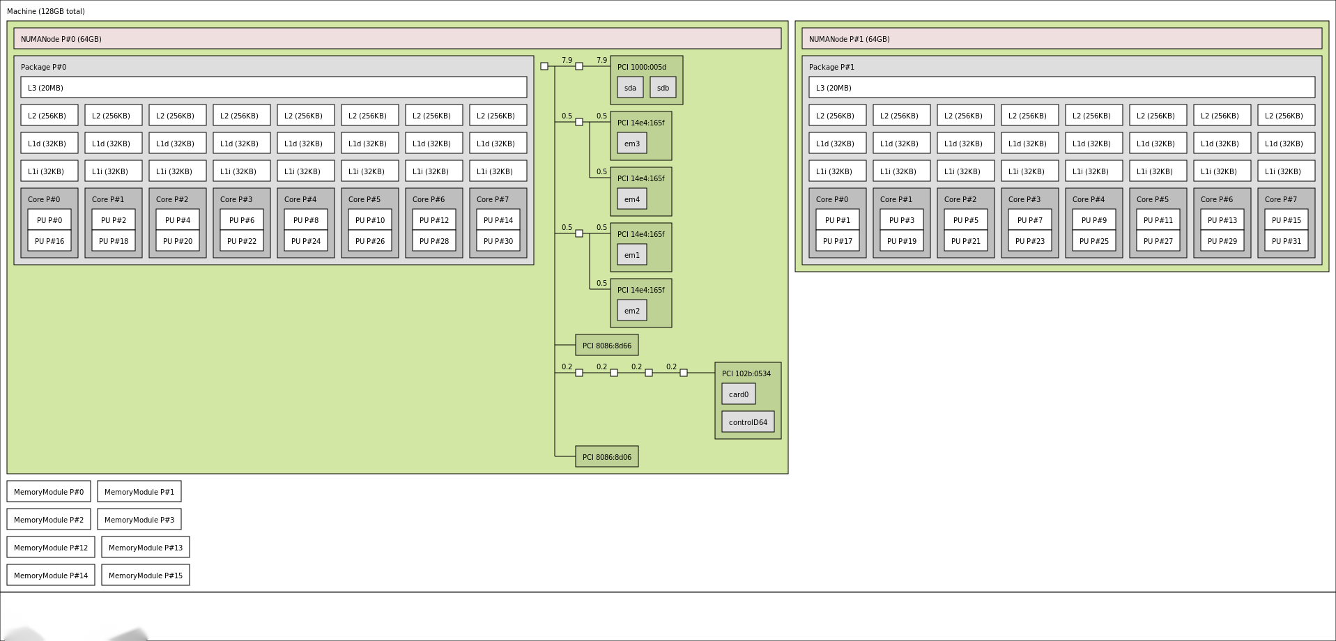
Displays the hardware topology
Displaying hardware topology can draw visual images through lstopo tool.
To install the lstopo tool:
yum install hwloc-libs hwloc-gui
Draw a hardware topology image:
lstopo --of png > machine.png
The results are shown in the figure below: